Mid Term Part (2): Individual Assignment: Tornado Diagrams and Bidding¶

By: Chengyi (Jeff) Chen

%load_ext autotime
%load_ext nb_black
%matplotlib inline
%config InlineBackend.figure_format = 'retina'

# Graphing
import matplotlib.pyplot as plt
import seaborn as sns

# Plotting Design Configs
sns.set(
    font="Verdana",
    rc={
        "axes.axisbelow": False,
        "axes.edgecolor": "lightgrey",
        "axes.facecolor": "None",
        "axes.grid": True,
        "grid.color": "lightgrey",
        "axes.labelcolor": "dimgrey",
        "axes.spines.right": False,
        "axes.spines.top": False,
        "figure.facecolor": "white",
        "lines.solid_capstyle": "round",
        "patch.edgecolor": "w",
        "patch.force_edgecolor": True,
        "text.color": "dimgrey",
        "xtick.bottom": False,
        "xtick.color": "dimgrey",
        "xtick.direction": "out",
        "xtick.top": False,
        "ytick.color": "dimgrey",
        "ytick.direction": "out",
        "ytick.left": False,
        "ytick.right": False,
        "figure.dpi": 100,
        "figure.figsize": (8, 6),
    },
)
sns.set_context(
    "notebook", rc={"font.size": 10, "axes.titlesize": 12, "axes.labelsize": 10}
)
sns.color_palette(palette="Spectral")

# General
import numpy as np
import scipy.stats as sp
import pandas as pd
from functools import partial

# Ignore warnings LOL
import warnings

warnings.simplefilter("ignore")

time: 1.22 s (started: 2021-04-02 15:44:56 +08:00)

def ρ(γ):
    """Risk tolerance"""
    return 1 / γ

time: 302 µs (started: 2021-04-02 15:44:57 +08:00)

def r(γ):
    """Risk Odds"""
    return np.log(γ)

time: 414 µs (started: 2021-04-02 15:44:57 +08:00)

def u(x, γ: np.array = np.array([0.0]), a: float = 0.0, b: float = 1.0):
    """Assuming user satisifies the Δ property, 
    calculates the U-values using either a 
    Piecewise Linear u = a + bx if γ = 0 (Risk-Neutral) 
    else Exponential u = a + be^(-xγ) U-curve U(x)
    
    Args:
        x (np.array): Payoffs of prospects matrix, Shape = (Number of deals, Number of prospects in each deal)
        γ (np.array): Risk-aversion coefficients, Shape = (Number of different risk-aversion coefficients for sensitivity analysis), Default = 0.0 (Risk-neutral) [γ > 0: Risk-averse, γ < 0: Risk-seeking]
        a (float): Constant for U-curve
        b (float): Coefficient for payoff variable
        
    Returns:
        np.array:
            U-values, Shape = (Number of Risk Aversion Coefficients γ, Number of deals, Number of prospects in each deal)
    """
    assert (
        x.ndim == 2
    ), "Payoffs require 2 dimensions, first dim is number of deals, second is number of prospects in each deal."
    γ = np.array([γ]) if np.isscalar(γ) else np.array(γ)
    return np.array(
        [
            np.apply_along_axis(
                func1d=lambda x, γ=γ: a + b * x if γ == 0 else a + b * np.exp(-x * γ),
                axis=-1,
                arr=x,
                γ=γ_i,
            )
            for γ_i in γ
        ]
    )

time: 627 µs (started: 2021-04-02 15:44:57 +08:00)

def eu(u, p):
    """Assuming user satisifies the Δ property, calculates the 
    hadamard product of the u values matrix and probabilities 
    matrix (respective probabilities associated with each 
    prospect in the u matrix)
    
    Args:
        u (np.array): U-values matrix, Shape = (Number of Risk Aversion Coefficients γ, Number of deals, Number of prospects in each deal)
        p (np.array): Probabilities of each prospect matrix, Shape = (Number of Risk Aversion Coefficients γ, Number of deals, Number of prospects in each deal)
        
    Returns:
        np.array:
            E-values, Shape = (Number of Risk Aversion Coefficients γ, Number of deals) 
    """
    assert (
        u.shape == p.shape
    ), "U-values matrix must be the same shape as the probabilities matrix."

    assert (
        u.ndim == 3
    ), "Both matrices must have 3 dimensions, Shape = (Number of Risk Aversion Coefficients γ, Number of deals, Number of prospects in each deal)."

    return np.sum(u * p, axis=-1)

time: 545 µs (started: 2021-04-02 15:44:57 +08:00)

def u_inv(eu, γ: np.array = np.array([0.0]), a: float = 0, b: float = 1):
    """Piecewise Inverse of Linear if γ = 0 (Risk-Neutral) 
    else Inverse of Exponential U-curve Certain equivalent 
    function U^{-1}(x)
    
    Args:
        eu (np.array): E[U-Values] / Expectation over u-values, AKA E-values, Shape = (Number of Risk Aversion Coefficients γ, Number of deals)
        γ (np.array): Risk-aversion coefficients, Shape = (Number of different risk-aversion coefficients for sensitivity analysis), Default = 0.0 (Risk-neutral) [γ > 0: Risk-averse, γ < 0: Risk-seeking]
        a (float): Constant for U-curve
        b (float): Coefficient for payoff variable
        
    Returns:
        np.array:
             Certainty Equivalent values, Shape = (Number of Risk Aversion Coefficients γ, Number of deals)
    """
    γ = np.array([γ]) if np.isscalar(γ) else np.array(γ)

    for eu_i, γ_i in zip(eu, γ):
        if not np.isclose(γ_i, 0):
            assert np.alltrue(
                eu_i > 0
            ), "E[U-Values] / Expectation over u-values must be positive for γ > 0 and γ < 0 in order for inverse of Exponential U-curve to work."

    assert (
        eu.shape[0] == γ.shape[0]
    ), "E-values first dimension must be the same as γ first dimension for inverse operation."

    return np.array(
        [
            list(
                map(
                    lambda eu, γ=γ_i: (eu - a) / b if γ == 0 else -(1 / γ) * np.log(eu),
                    eu_i,
                )
            )
            for eu_i, γ_i in zip(eu, γ)
        ]
    )

time: 839 µs (started: 2021-04-02 15:44:57 +08:00)

def certainty_equivalent_values_calculator(
    u,
    u_inv,
    x: np.array = None,
    p: np.array = None,
    N: int = 10,
    payout_lb: float = 0.0,
    payout_ub: float = 100.0,
    γ: np.array = np.array([0.0]),
):
    """Assuming user satisifies the Δ property, calculates the Certainty Equivalent values for a given 
    payoff matrix `x` and probability matrix `p`. If both matrices
    are not provided, random matrices will be sampled to simulate
    calculations.

    Args:
        u (function): U-curve function
        u_inv (function): Inverse U-curve function
        x (np.array): Payoffs of prospects matrix, Shape = (Number of deals, Number of prospects in each deal)
        p (np.array): Probabilities of each prospect matrix, Shape = (Number of deals, Number of prospects in each deal)
        N (int): Number of prospects
        payout_lb (float): Lower Bound of Payout for simulation, Default = 0.0
        payout_ub (float): Upper Bound of Payout for simulation, Default = 100.0
        γ (np.array): Risk-aversion coefficients, Shape = (Number of different risk-aversion coefficients for sensitivity analysis), Default = 0.0 (Risk-neutral) [γ > 0: Risk-averse, γ < 0: Risk-seeking]
        
    Returns:
        np.array:
            Certainty Equivalent values, Shape = (Number of Risk Aversion Coefficients γ, Number of deals)
    """
    γ = np.array([γ]) if np.isscalar(γ) else np.array(γ)

    # Case 1: Simulator - Both x and p arent provided
    if p is None and x is None:

        # Preferential probabilities for each prospect
        p = np.random.dirichlet(np.ones(N), size=1)

        # Payouts for each prospect
        x = np.expand_dims(np.random.randint(payout_lb, payout_ub, size=N), axis=0)

    # Case 2: Simulator - Only payouts provided
    elif p is None:

        # Payouts for each prospect
        x = np.expand_dims(
            np.random.randint(payout_lb, payout_ub, size=p.shape[-1]), axis=0
        )

    # Case 3: Simulator - Only probabilities provided
    elif x is None:

        # Preferential probabilities for each prospect
        p = np.random.dirichlet(np.ones(x.shape[-1]), size=1)

    # Case 4: Calculator - Both are provided
    else:

        pass

    # Check that payoffs and probability assignments are the same shape
    assert (
        x.shape == p.shape
    ), "Payoffs `x` and Probabilities `p` must be the same shape=(Number of deals, Number of prospects in each deal)."

    # Calculates U-values Shape = (Number of Risk Aversion Coefficients γ, Number of deals, Number of prospects in each deal)
    u_values = u(x, γ=γ)

    # Reshape p to match U-values shape
    p_reshaped = np.array([p for _ in range(u_values.shape[0])])

    # Expectation of U values Shape = (Number of Risk Aversion Coefficients γ, Number of deals)
    eu_values = eu(u=u_values, p=p_reshaped)

    # Certainty equivalent value of deal
    ce_values = u_inv(eu_values, γ=γ)

    return ce_values

time: 1.23 ms (started: 2021-04-02 15:44:57 +08:00)

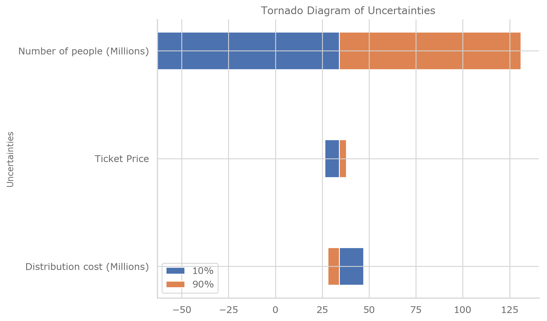
1) Tornado Diagrams: The Clairvoyant goes to College¶

Flicks Inc is a major entertainment corporation. They have just produced a major motion picture called The Clairvoyant goes to College. They have spent some money on the movie and they believe their future profit is calculated as

(37)¶\[\begin{align} \text{Profit} &= \left(0.2\times \text{Number of people} \times \text{Ticket price}\right) - \text{Distribution cost} \\ \end{align}\]

They provide the following 10-50-90 assessments for three uncertainties. (Distribution cost and Number people seeing movie is in millions of $\$ $ while ticket price is in $\$ $)

Draw the tornado diagram and show all tables used in the calculations.

clairvoyant_goes_to_college_uncertainties = pd.DataFrame(
    data=[[11.33, 76.0, 140.66], [7.0, 7.5, 7.75], [67.0, 80.0, 86.0]],
    index=[
        "Number of people (Millions)",
        "Ticket Price",
        "Distribution cost (Millions)",
    ],
    columns=["10%", "50%", "90%"],
)
clairvoyant_goes_to_college_uncertainties

	10%	50%	90%
Number of people (Millions)	11.33	76.0	140.66
Ticket Price	7.00	7.5	7.75
Distribution cost (Millions)	67.00	80.0	86.00

time: 10.3 ms (started: 2021-04-02 15:44:57 +08:00)

# Profit Formula (Millions)
profit = lambda n_ppl, ticket_px, dist_cost: (0.2 * n_ppl * ticket_px) - dist_cost

time: 370 µs (started: 2021-04-02 15:44:57 +08:00)

# Get the Profit, fixing entries and using baseline (50%) values as other parameters
npv = clairvoyant_goes_to_college_uncertainties.copy()
for row in clairvoyant_goes_to_college_uncertainties.index:
    for col in clairvoyant_goes_to_college_uncertainties.columns:
        profit_params = clairvoyant_goes_to_college_uncertainties["50%"].copy()
        profit_params[row] = clairvoyant_goes_to_college_uncertainties[col][row]
        npv[col][row] = profit(*profit_params)

npv

	10%	50%	90%
Number of people (Millions)	-63.005	34.0	130.99
Ticket Price	26.400	34.0	37.80
Distribution cost (Millions)	47.000	34.0	28.00

time: 10.1 ms (started: 2021-04-02 15:44:57 +08:00)

# Max Swing
max_swing = npv.max(axis=1) - npv.min(axis=1)
max_swing

Number of people (Millions)     193.995
Ticket Price                     11.400
Distribution cost (Millions)     19.000
dtype: float64

time: 6.65 ms (started: 2021-04-02 15:44:57 +08:00)

# Max Swing Squared
max_swing_squared = max_swing ** 2
max_swing_squared

Number of people (Millions)     37634.060025
Ticket Price                      129.960000
Distribution cost (Millions)      361.000000
dtype: float64

time: 2.8 ms (started: 2021-04-02 15:44:57 +08:00)

# Normalized Max Swing Squared
norm_max_swing_squared = max_swing_squared / sum(max_swing_squared)
norm_max_swing_squared

Number of people (Millions)     0.987122
Ticket Price                    0.003409
Distribution cost (Millions)    0.009469
dtype: float64

time: 3.32 ms (started: 2021-04-02 15:44:57 +08:00)

# Tornado diagram
npv = npv.reindex(norm_max_swing_squared.index[::-1])

fig, ax = plt.subplots()

ax.barh(
    npv.index,
    npv["50%"].values - npv["10%"].values,
    0.35,
    align="center",
    label="10%",
    left=npv["10%"].values,
)
ax.barh(
    npv.index,
    npv["90%"].values - npv["50%"].values,
    0.35,
    align="center",
    label="90%",
    left=npv["50%"].values,
)

ax.set_ylabel("Uncertainties")
ax.set_title("Tornado Diagram of Uncertainties")
ax.legend()

plt.show()

time: 311 ms (started: 2021-04-02 15:44:57 +08:00)

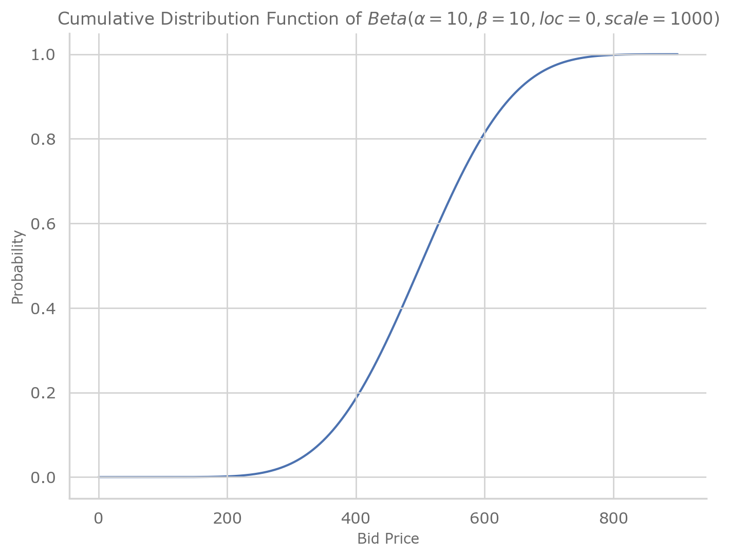
2) Optimal Bidding¶

Determine the optimal bid for a decision maker with an exponential $u$-function with a risk aversion coefficient, $\gamma = 0.001$, a maximum competitive bid distribution, as a scaled Beta distribution, $Beta\left(\alpha=10, \beta=10, \text{loc}=0, \text{scale}=1000\right)$, and PIBP for the bidding item is $ \$ 900$.

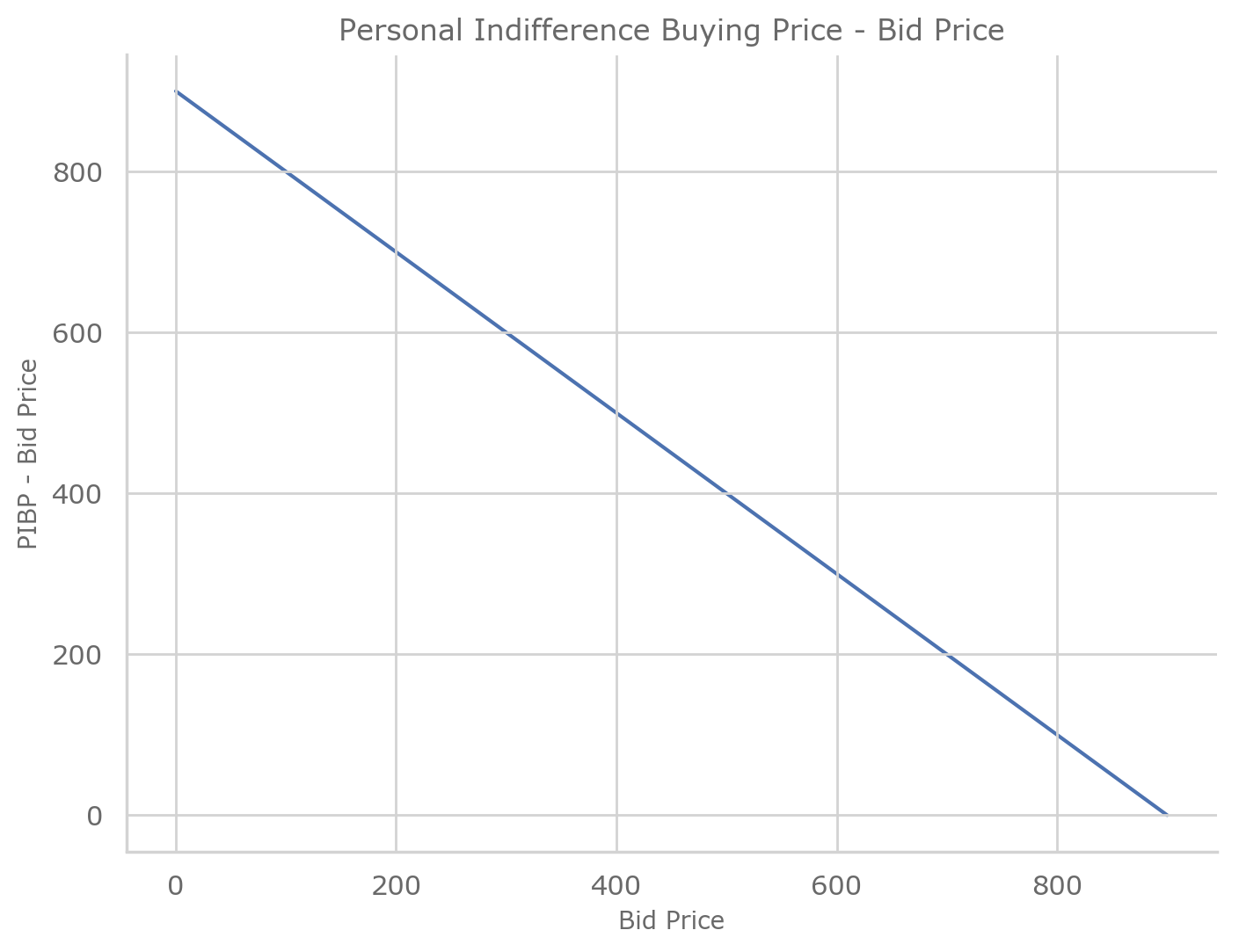
Plot the Opposing forces of bidding (i.e. plot the CDF and the curve of [PIBP-bid])

pibp = 900
γ = 0.001
bids = np.array(list(range(900 + 1)))
pibp_net = pibp - bids
p_acquire = np.array([sp.beta.cdf(x=rv, a=10, b=10, loc=0, scale=1000) for rv in bids])

time: 202 ms (started: 2021-04-02 15:44:58 +08:00)

fig, ax = plt.subplots(1, 1)

ax.plot(bids, p_acquire)
ax.set_xlabel("Bid Price")
ax.set_ylabel("Probability")
ax.set_title(
    r"Cumulative Distribution Function of $Beta \left(\alpha=10, \beta=10, loc=0, scale=1000 \right)$"
)
plt.show()

time: 483 ms (started: 2021-04-02 15:44:58 +08:00)

fig, ax = plt.subplots(1, 1)

ax.plot(bids, pibp_net)
ax.set_xlabel("Bid Price")
ax.set_ylabel("PIBP - Bid Price")
ax.set_title(r"Personal Indifference Buying Price - Bid Price")
plt.show()

time: 271 ms (started: 2021-04-02 15:44:58 +08:00)

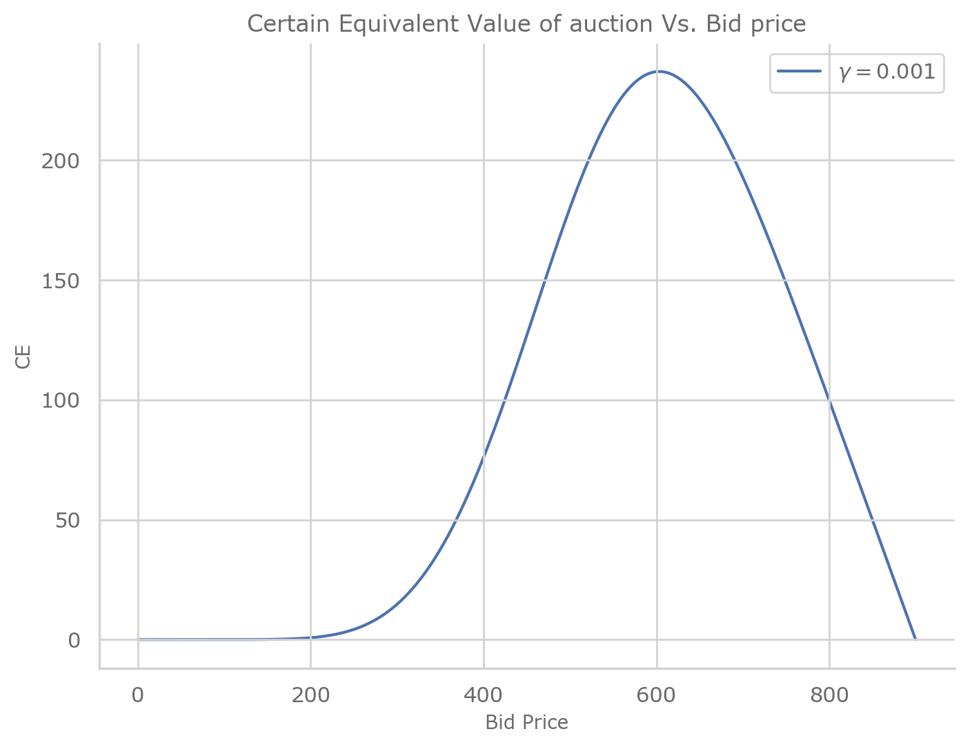
Plot the value of the auction situation (certain equivalent) vs the bid amount.

fig, ax = plt.subplots(1, 1)

ax.plot(
    bids,
    certainty_equivalent_values_calculator(
        u=partial(u, γ=np.array([γ]), a=0, b=1),
        u_inv=partial(u_inv, γ=np.array([γ]), a=0, b=1),
        x=np.vstack((pibp_net, np.zeros(pibp_net.shape))).T,
        p=np.vstack((p_acquire, 1 - p_acquire)).T,
        γ=np.array([γ]),
    )[0],
    label=r"$\gamma = 0.001$",
)
ax.set_xlabel("Bid Price")
ax.set_ylabel("CE")
ax.set_title(r"Certain Equivalent Value of auction Vs. Bid price")
plt.legend()
plt.show()

time: 293 ms (started: 2021-04-02 15:44:59 +08:00)

Determine the least amount the decision maker needs to be paid in order to not participate in this bidding situation.

certainty_equivalent_auction_values = np.round(
    certainty_equivalent_values_calculator(
        u=partial(u, γ=0.001, a=0, b=1),
        u_inv=partial(u_inv, γ=0.001, a=0, b=1),
        x=np.vstack((pibp_net, np.zeros(pibp_net.shape))).T,
        p=np.vstack((p_acquire, 1 - p_acquire)).T,
        γ=0.001,
    )[0],
    2,
)

print(
    "The minimum amount the decision maker needs to be paid in order to not participate in the bidding is: ${}".format(
        np.min(
            certainty_equivalent_auction_values[
                np.nonzero(certainty_equivalent_auction_values)
            ]
        )
    )
)

The minimum amount the decision maker needs to be paid in order to not participate in the bidding is: $0.01
time: 15.8 ms (started: 2021-04-02 15:44:59 +08:00)

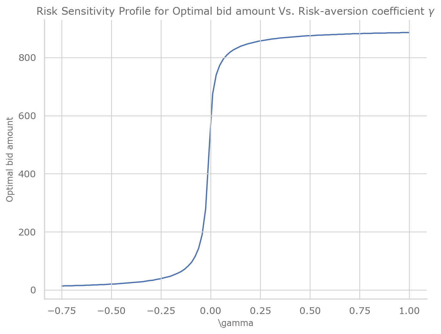
Plot a sensitivity analysis for the optimal bid vs. the risk aversion coefficient.

fig, ax = plt.subplots(1, 1)

γ = np.linspace(-0.75, 1, num=100)

ax.plot(
    γ,
    [
        bids[optimal_bid_idx_for_γ]
        for optimal_bid_idx_for_γ in np.argmax(
            certainty_equivalent_values_calculator(
                u=partial(u, γ=γ, a=0, b=1),
                u_inv=partial(u_inv, γ=γ, a=0, b=1),
                x=np.vstack((pibp_net, np.zeros(pibp_net.shape))).T,
                p=np.vstack((p_acquire, 1 - p_acquire)).T,
                γ=γ,
            ),
            axis=1,
        )
    ],
)
ax.set_xlabel(r"\gamma")
ax.set_ylabel("Optimal bid amount")
ax.set_title(
    r"Risk Sensitivity Profile for Optimal bid amount Vs. Risk-aversion coefficient $\gamma$"
)
plt.show()

time: 1.13 s (started: 2021-04-02 15:44:59 +08:00)

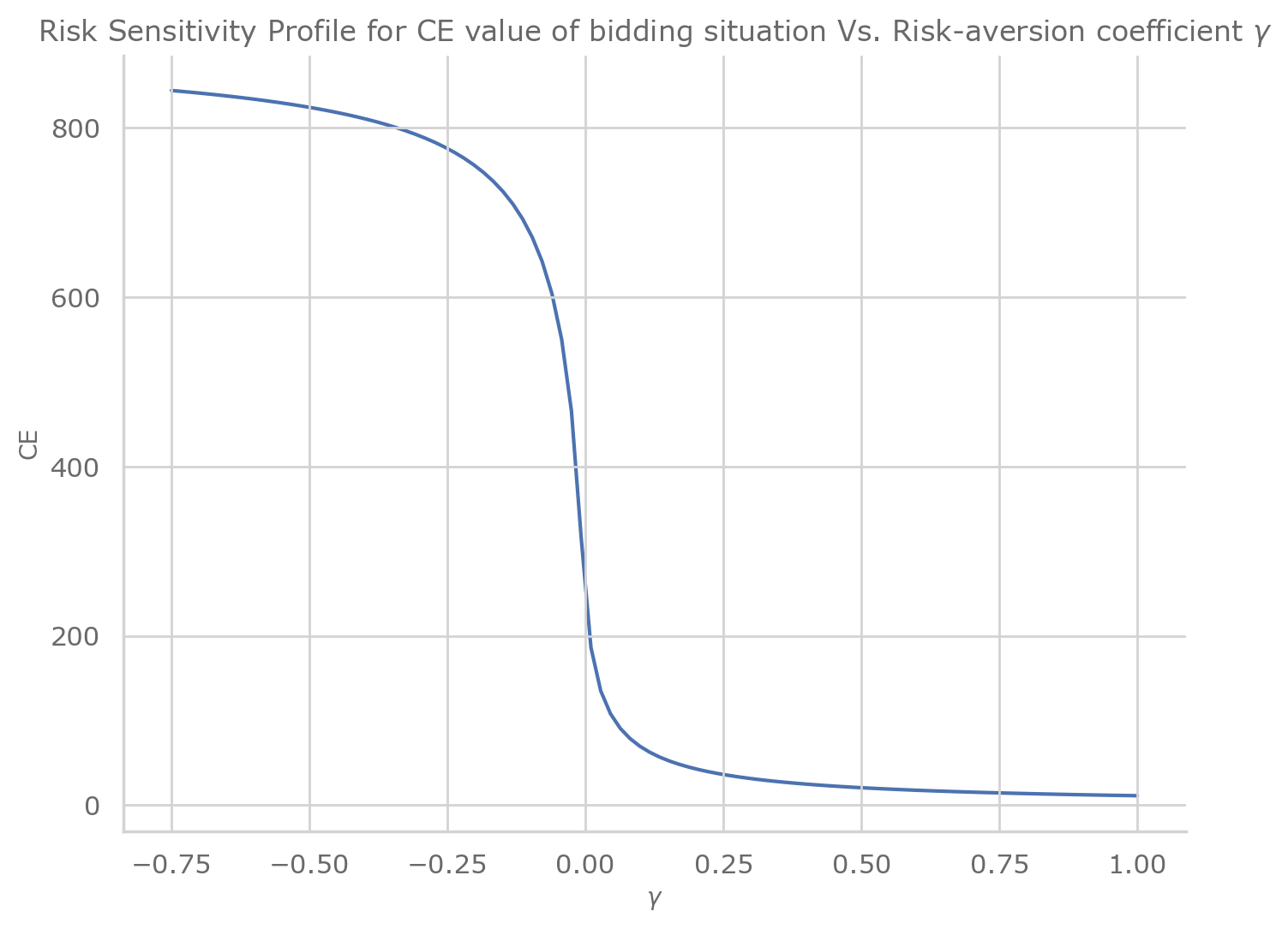
Plot a sensitivity analysis for value of bidding situation vs the risk aversion coefficient.

fig, ax = plt.subplots(1, 1)

γ = np.linspace(-0.75, 1, num=100)

ax.plot(
    γ,
    np.max(
        certainty_equivalent_values_calculator(
            u=partial(u, γ=γ, a=0, b=1),
            u_inv=partial(u_inv, γ=γ, a=0, b=1),
            x=np.vstack((pibp_net, np.zeros(pibp_net.shape))).T,
            p=np.vstack((p_acquire, 1 - p_acquire)).T,
            γ=γ,
        ),
        axis=1,
    ),
)
ax.set_xlabel(r"$\gamma$")
ax.set_ylabel("CE")
ax.set_title(
    "Risk Sensitivity Profile for CE value of bidding situation Vs. Risk-aversion coefficient $\gamma$"
)
plt.show()

time: 997 ms (started: 2021-04-02 15:45:00 +08:00)

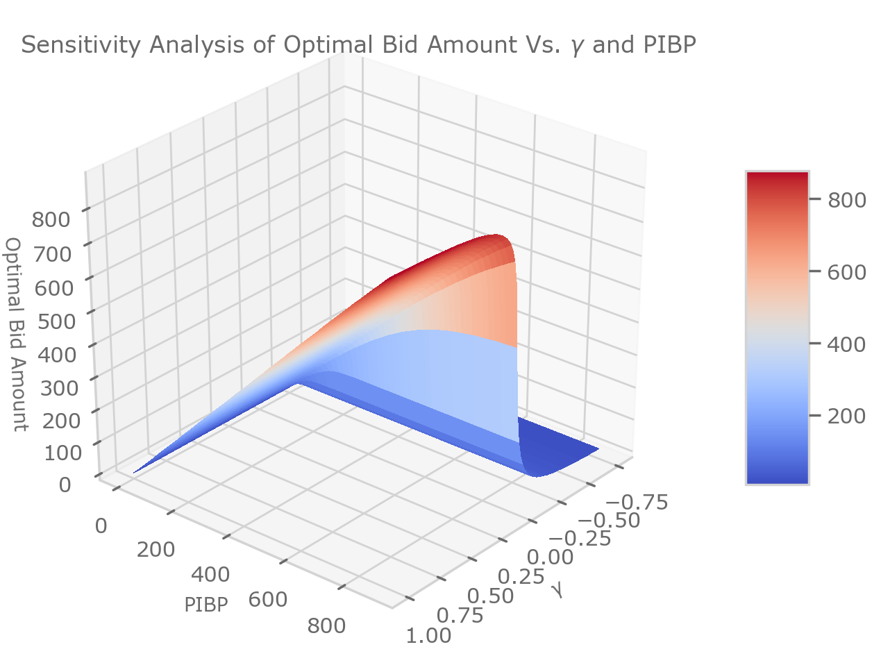
Extra Credit: Plot a two-way sensitivity analysis for optimal bid vs the two parameters (risk aversion coefficient and PIBP). This is a 3D plot.

from mpl_toolkits.mplot3d import Axes3D
from matplotlib import cm, colors
from matplotlib.ticker import LinearLocator

fig, ax = plt.subplots(subplot_kw={"projection": "3d"})

bids = np.array(list(range(900 + 1)))
p_acquire = np.array([sp.beta.cdf(x=rv, a=10, b=10, loc=0, scale=1000) for rv in bids])
γ = np.linspace(-0.75, 1, num=100)
pibp_values = np.linspace(0, 900 + 1)
X, Y = np.meshgrid(γ, pibp_values)
Z = np.array(
    [
        [
            bids[
                np.argmax(
                    certainty_equivalent_values_calculator(
                        u=partial(u, γ=γ_i, a=0, b=1),
                        u_inv=partial(u_inv, γ=γ_i, a=0, b=1),
                        x=np.vstack((pibp - bids, np.zeros(bids.shape))).T,
                        p=np.vstack((p_acquire, 1 - p_acquire)).T,
                        γ=γ_i,
                    ),
                    axis=1,
                )[0]
            ]
            for γ_i in γ
        ]
        for pibp in pibp_values
    ]
)

# Plot the surface.
surf = ax.plot_surface(X, Y, Z, cmap=cm.coolwarm, linewidth=0, antialiased=False,)
ax.view_init(30, 40)
ax.set_xlabel(r"$\gamma$")
ax.set_ylabel(r"PIBP")
ax.set_zlabel("Optimal Bid Amount")
ax.set_title("Sensitivity Analysis of Optimal Bid Amount Vs. $\gamma$ and PIBP")

# Add a color bar which maps values to colors.
fig.colorbar(surf, shrink=0.5, aspect=5)

plt.show()

time: 39.2 s (started: 2021-04-02 15:45:01 +08:00)

ΨΦ

Mid Term Part (2): Individual Assignment: Tornado Diagrams and Bidding¶

1) Tornado Diagrams: The Clairvoyant goes to College¶

2) Optimal Bidding¶