
Project 2: Carry
By: Chengyi (Jeff) Chen
Description of The Project:
We want to build a commodity curve strategy by trading WTI futures. The commodity curve strategy takes a long position of an optimally-chosen contract and a short position of another contract at any time in order to capture the commodity’s term struture premium.
Here are the steps for portfolio construction and rebalancing:
Step 1: At each month-end date, we consider contracts on tenors from T2 to T12. (T1 contract would not be considered since it has less than 1 month to expiration)
Step 2A: For each tenor contract, calculate the expected rolling return if holding the contract for one month based on the current term structure. (Let’s assume the expiration dates of two adjacent contracts are always exactly one-month away).
Step 2B: Among the 11 contracts (from T2 to T12), build a portfolio with one long position in the contract with the highest expected rolling return, and one short position in the contract with the lowest expected rolling return.
Step 3: Hold the portfolio till the next month-end and rebalance the portfolio.
You need to run the back-test for the strategy from 1/31/2000 to 1/31/2019, calculate the strategy’s monthly returns, and deliver the following results:
Assume we invest \$1 in the strategy from day 1, i.e., 1/31/2000, please plot the value of our investment over time.
Calculate the strategy’s calendar year returns, i.e., cumulative returns in each year from 2000 to 2019.
Calculate the annualized return, annualized risk, and Sharpe ratio (let’s assume risk-free rate of 0) of the strategy.
Identify the maximum drawdown period for this strategy.
%load_ext autotime
%load_ext nb_black
%matplotlib inline

import matplotlib.pyplot as plt

# from mpl_toolkits.mplot3d import Axes3D

plt.rcParams["figure.dpi"] = 300
plt.rcParams["figure.figsize"] = (10, 8)

from collections import defaultdict
from datetime import datetime
import pandas as pd
import numpy as np
import cvxpy as cp
import scipy as sp
import plotly.express as px
import plotly.graph_objects as go
Data
raw_data = pd.read_excel("./data/Project2_WTI_OilCurve.XLSX", sheet_name=1, header=None)


def format_commodity_prices(df):
    new_df = df.iloc[2:, 1:4]
    new_df.columns = df.iloc[1, 1:4].values
    new_df.index = df.iloc[2:, 0].values
    return new_df


commodity_data = pd.concat(
    [
        format_commodity_prices(raw_data.iloc[:, start:stop])
        for start, stop in zip(
            list(range(0, raw_data.shape[1] + 1, 6)),
            list(range(5, raw_data.shape[1] + 1, 6)),
        )
    ],
    axis=1,
    keys=[f"Term {idx+1}" for idx in range(12)],
)

commodity_data.index = pd.to_datetime(commodity_data.index)
commodity_data.head()
| Term 1 | Term 2 | Term 3 | Term 4 | ... | Term 9 | Term 10 | Term 11 | Term 12 | |||||||||||||
|---|---|---|---|---|---|---|---|---|---|---|---|---|---|---|---|---|---|---|---|---|---|
| FUT_CUR_GEN_TICKER | PX LAST | VOLUME | FUT_CUR_GEN_TICKER | PX LAST | VOLUME | FUT_CUR_GEN_TICKER | PX LAST | VOLUME | FUT_CUR_GEN_TICKER | ... | VOLUME | FUT_CUR_GEN_TICKER | PX LAST | VOLUME | FUT_CUR_GEN_TICKER | PX LAST | VOLUME | FUT_CUR_GEN_TICKER | PX LAST | VOLUME | |
| 2000-01-31 | CLH00 | 27.64 | 83938 | CLJ00 | 26.72 | 30986 | CLK00 | 25.97 | 6006 | CLM00 | ... | 781 | CLZ00 | 22.49 | 5380 | CLF01 | 22.14 | 1354 | CLG01 | 21.81 | 848 |
| 2000-02-01 | CLH00 | 28.22 | 80801 | CLJ00 | 27.26 | 33388 | CLK00 | 26.49 | 7648 | CLM00 | ... | 718 | CLZ00 | 22.84 | 8690 | CLF01 | 22.47 | 1354 | CLG01 | 22.12 | 580 |
| 2000-02-02 | CLH00 | 27.55 | 100243 | CLJ00 | 26.67 | 50618 | CLK00 | 25.96 | 9423 | CLM00 | ... | 716 | CLZ00 | 22.55 | 5921 | CLF01 | 22.18 | 771 | CLG01 | 21.83 | 28 |
| 2000-02-03 | CLH00 | 28.03 | 80492 | CLJ00 | 27.13 | 38659 | CLK00 | 26.39 | 11135 | CLM00 | ... | 4071 | CLZ00 | 22.95 | 3372 | CLF01 | 22.57 | 3856 | CLG01 | 22.21 | 225 |
| 2000-02-04 | CLH00 | 28.82 | 67793 | CLJ00 | 27.82 | 27438 | CLK00 | 27.04 | 9120 | CLM00 | ... | 197 | CLZ00 | 23.41 | 3458 | CLF01 | 23.03 | 281 | CLG01 | 22.67 | 106 |
5 rows × 36 columns
time: 2.6 s
Step 1: At each month-end date, we consider contracts on tenors from T2 to T12. (T1 contract would not be considered since it has less than 1 month to expiration)
contracts_of_interest = commodity_data[commodity_data.index.is_month_end].loc[
    :, [(f"Term {idx}", "PX LAST") for idx in range(1, 13)]
]
contracts_of_interest.head()
| Term 1 | Term 2 | Term 3 | Term 4 | Term 5 | Term 6 | Term 7 | Term 8 | Term 9 | Term 10 | Term 11 | Term 12 | |
|---|---|---|---|---|---|---|---|---|---|---|---|---|
| PX LAST | PX LAST | PX LAST | PX LAST | PX LAST | PX LAST | PX LAST | PX LAST | PX LAST | PX LAST | PX LAST | PX LAST | |
| 2000-01-31 | 27.64 | 26.72 | 25.97 | 25.32 | 24.71 | 24.17 | 23.71 | 23.27 | 22.87 | 22.49 | 22.14 | 21.81 |
| 2000-02-29 | 30.43 | 28.85 | 27.68 | 26.74 | 26 | 25.35 | 24.79 | 24.32 | 23.88 | 23.44 | 23.04 | 22.65 |
| 2000-03-31 | 26.9 | 26.38 | 26.04 | 25.76 | 25.48 | 25.19 | 24.9 | 24.6 | 24.28 | 23.97 | 23.68 | 23.39 |
| 2000-05-31 | 29.01 | 28.42 | 27.89 | 27.4 | 26.92 | 26.47 | 26.06 | 25.69 | 25.32 | 24.95 | 24.58 | 24.21 |
| 2000-06-30 | 32.5 | 31.13 | 30.2 | 29.51 | 28.94 | 28.42 | 27.92 | 27.45 | 27.02 | 26.61 | 26.23 | 25.87 |
time: 21.7 ms
unstacked_price = (
    (
        commodity_data[commodity_data.index.is_month_end].loc[
            :, [(f"Term {idx}", "PX LAST") for idx in range(1, 13)]
        ]
    )
    .unstack()
    .reset_index()
    .drop(["level_1"], axis=1)
)

unstacked_volume = (
    (
        commodity_data[commodity_data.index.is_month_end].loc[
            :, [(f"Term {idx}", "VOLUME") for idx in range(1, 13)]
        ]
    )
    .unstack()
    .reset_index()
    .drop(["level_1"], axis=1)
)

unstacked = pd.merge(unstacked_price, unstacked_volume, on=["level_0", "level_2"])
unstacked.columns = ["term", "date", "price", "volume"]
unstacked["price"] = unstacked["price"].astype(float)
unstacked["volume"] = unstacked["volume"].astype(int)
unstacked["term"] = unstacked["term"].apply(
    lambda x: int(x.lower().replace("term ", ""))
)
unstacked["date"] = unstacked["date"].astype(str)
fig = px.scatter(
    data_frame=unstacked,
    x="term",
    y="price",
    size="volume",
    animation_frame="date",
    range_x=[0, 13],
    range_y=[unstacked["price"].min(), unstacked["price"].max()],
    title="Futures Curve for WTI",
)
fig.show()
time: 5.94 s
Step 2A: For each tenor contract, calculate the expected rolling return if holding the contract for one month based on the current term structure. (Let’s assume the expiration dates of two adjacent contracts are always exactly one-month away).
expected_rolling_return_assume_current_term_structure = (
    contracts_of_interest.pct_change(periods=-1, axis=1).shift(1, axis=1).dropna(axis=1)
)
expected_rolling_return_assume_current_term_structure.head()
| Term 2 | Term 3 | Term 4 | Term 5 | Term 6 | Term 7 | Term 8 | Term 9 | Term 10 | Term 11 | Term 12 | |
|---|---|---|---|---|---|---|---|---|---|---|---|
| PX LAST | PX LAST | PX LAST | PX LAST | PX LAST | PX LAST | PX LAST | PX LAST | PX LAST | PX LAST | PX LAST | |
| 2000-01-31 | 0.034431 | 0.028879 | 0.025671 | 0.024686 | 0.022342 | 0.019401 | 0.018908 | 0.017490 | 0.016896 | 0.015808 | 0.015131 |
| 2000-02-29 | 0.054766 | 0.042269 | 0.035153 | 0.028462 | 0.025641 | 0.022590 | 0.019326 | 0.018425 | 0.018771 | 0.017361 | 0.017219 |
| 2000-03-31 | 0.019712 | 0.013057 | 0.010870 | 0.010989 | 0.011513 | 0.011647 | 0.012195 | 0.013180 | 0.012933 | 0.012247 | 0.012398 |
| 2000-05-31 | 0.020760 | 0.019003 | 0.017883 | 0.017831 | 0.017000 | 0.015733 | 0.014402 | 0.014613 | 0.014830 | 0.015053 | 0.015283 |
| 2000-06-30 | 0.044009 | 0.030795 | 0.023382 | 0.019696 | 0.018297 | 0.017908 | 0.017122 | 0.015914 | 0.015408 | 0.014487 | 0.013916 |
time: 42.1 ms
Step 2B: Among the 11 contracts (from T2 to T12), build a portfolio with one long position in the contract with the highest expected rolling return, and one short position in the contract with the lowest expected rolling return.
# actual_returns = contracts_of_interest.pct_change().shift(-1).dropna()
longs = expected_rolling_return_assume_current_term_structure.idxmax(axis=1)
# longs = longs.to_frame().reset_index()
# longs.columns = ["date", "term"]
shorts = expected_rolling_return_assume_current_term_structure.idxmin(axis=1)
# shorts.to_frame().reset_index()
# shorts.columns = ["date", "term"]
time: 11.5 ms
Step 3: Hold the portfolio till the next month-end and rebalance the portfolio.
longs_buy_price = (
    longs.reset_index()
    .rename({"index": "date", 0: "term"}, axis=1)
    .apply(lambda row: contracts_of_interest.loc[row["date"], row["term"]], axis=1)[:-1]
)  # Exclude last buy price since we can't observe how much the next month sell price is

longs_sell_price = (
    longs.shift(1)
    .dropna()
    .reset_index()
    .rename({"index": "date", 0: "term"}, axis=1)
    .apply(
        lambda row: contracts_of_interest.loc[
            row["date"],
            ("Term " + str(int(row["term"][0].split(" ")[1]) - 1), row["term"][1]),
        ],  # Get the contract price @ term = t - 1 month
        axis=1,
    )
)

longs_returns = (longs_sell_price / longs_buy_price) - 1
longs_returns.index = longs.index[1:]
longs_returns
2000-02-29    0.138847
2000-03-31   -0.067591
2000-05-31    0.099697
2000-06-30    0.143561
2000-07-31   -0.118856
                ...
2018-08-31    0.032086
2018-10-31   -0.058527
2018-11-30   -0.210238
2018-12-31   -0.069830
2019-01-31    0.130722
Length: 164, dtype: float64
time: 116 ms
shorts_buy_price = (
    shorts.reset_index()
    .rename({"index": "date", 0: "term"}, axis=1)
    .apply(lambda row: contracts_of_interest.loc[row["date"], row["term"]], axis=1)[:-1]
)  # Exclude last buy price since we can't observe how much the next month sell price is

shorts_sell_price = (
    shorts.shift(1)
    .dropna()
    .reset_index()
    .rename({"index": "date", 0: "term"}, axis=1)
    .apply(
        lambda row: contracts_of_interest.loc[
            row["date"],
            ("Term " + str(int(row["term"][0].split(" ")[1]) - 1), row["term"][1]),
        ],  # Get the contract price @ term = t - 1 month
        axis=1,
    )
)

shorts_returns = 1 - (shorts_sell_price / shorts_buy_price)
shorts_returns.index = shorts.index[1:]
shorts_returns
2000-02-29   -0.056396
2000-03-31   -0.045475
2000-05-31   -0.082686
2000-06-30   -0.086804
2000-07-31    0.017395
                ...
2018-08-31   -0.031180
2018-10-31    0.046664
2018-11-30    0.220599
2018-12-31    0.111176
2019-01-31   -0.167706
Length: 164, dtype: float64
time: 93.7 ms
monthly_strategy_returns = pd.concat(
    [longs_returns, shorts_returns], keys=["longs", "shorts"], axis=1
)
monthly_strategy_returns
| longs | shorts | |
|---|---|---|
| 2000-02-29 | 0.138847 | -0.056396 |
| 2000-03-31 | -0.067591 | -0.045475 |
| 2000-05-31 | 0.099697 | -0.082686 |
| 2000-06-30 | 0.143561 | -0.086804 |
| 2000-07-31 | -0.118856 | 0.017395 |
| ... | ... | ... |
| 2018-08-31 | 0.032086 | -0.031180 |
| 2018-10-31 | -0.058527 | 0.046664 |
| 2018-11-30 | -0.210238 | 0.220599 |
| 2018-12-31 | -0.069830 | 0.111176 |
| 2019-01-31 | 0.130722 | -0.167706 |
164 rows × 2 columns
time: 6.88 ms
portfolio_returns = (
    monthly_strategy_returns.sum(axis=1)
    .to_frame()
    .rename({0: "monthly_returns"}, axis=1)
)
portfolio_returns.head()
| monthly_returns | |
|---|---|
| 2000-02-29 | 0.082451 |
| 2000-03-31 | -0.113066 |
| 2000-05-31 | 0.017010 |
| 2000-06-30 | 0.056757 |
| 2000-07-31 | -0.101462 |
time: 4.98 ms
You need to run the back-test for the strategy from 1/31/2000 to 1/31/2019, calculate the strategy’s monthly returns, and deliver the following results:
Assume we invest \$1 in the strategy from day 1, i.e., 1/31/2000, please plot the value of our investment over time.
Calculate the strategy’s calendar year returns, i.e., cumulative returns in each year from 2000 to 2019.
Calculate the annualized return, annualized risk, and Sharpe ratio (let’s assume risk-free rate of 0) of the strategy.
Identify the maximum drawdown period for this strategy.
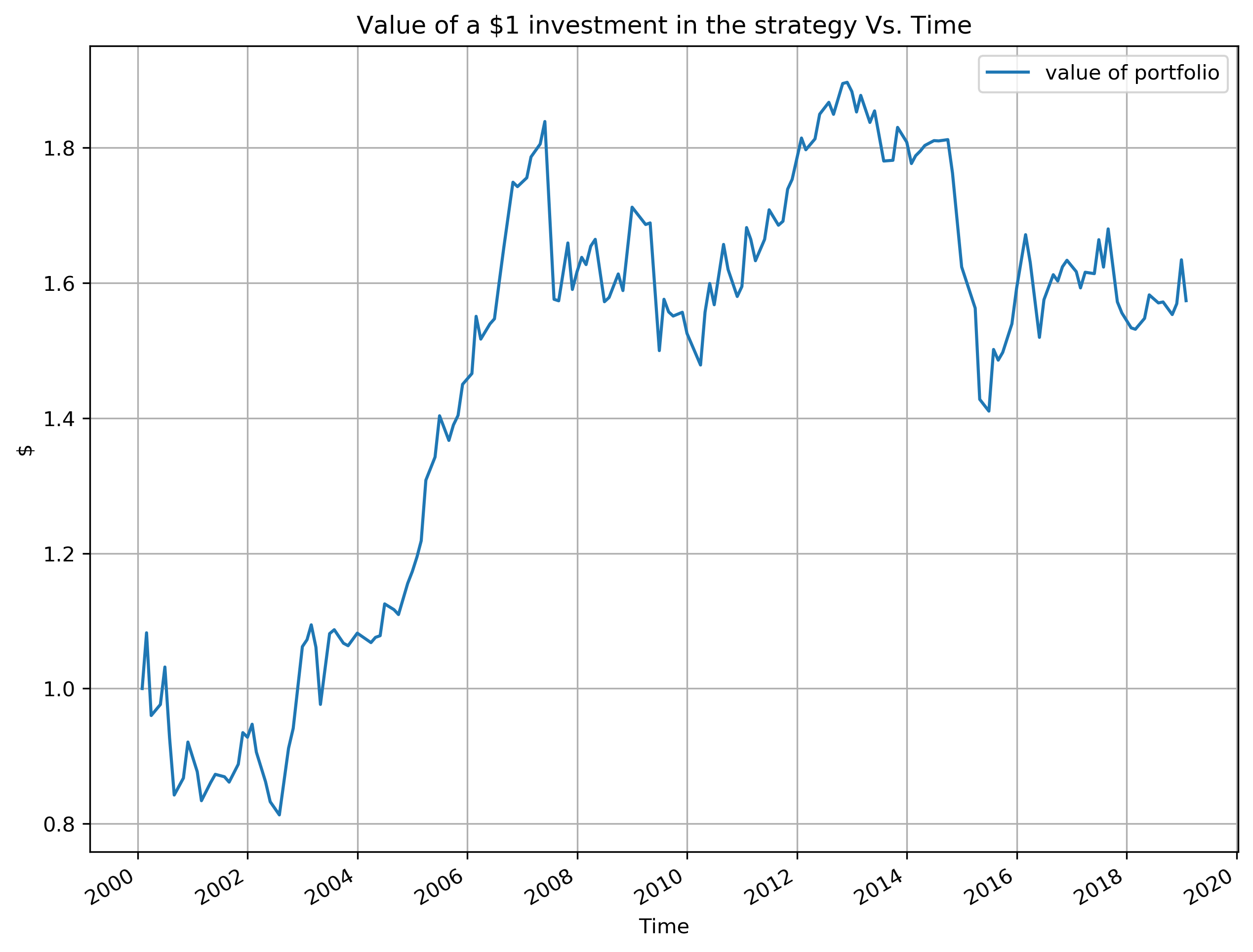
1. Assume we invest \$1 in the strategy from day 1, i.e., 1/31/2000, please plot the value of our investment over time.
fig, ax = plt.subplots(1, 1)
portfolio_value = pd.concat(
    [
        pd.DataFrame({"monthly_returns": 1}, index=[contracts_of_interest.index[0]]),
        (portfolio_returns + 1).cumprod(),
    ],
    axis=0,
).rename({"monthly_returns": "value of portfolio"}, axis=1)
portfolio_value.plot(ax=ax)
ax.set_xlabel("Time")
ax.set_ylabel("$")
ax.set_title("Value of a $1 investment in the strategy Vs. Time")
plt.legend()
plt.grid(True)
plt.show()
time: 637 ms
2. Calculate the strategy’s calendar year returns, i.e., cumulative returns in each year from 2000 to 2019.
portfolio_returns["year"] = portfolio_returns.index.year
portfolio_returns.groupby(by="year")["monthly_returns"].apply(
    lambda returns: np.prod(1 + returns) ** (12 / len(returns)) - 1
).to_frame().rename({"monthly_returns": "calendar_year_returns"}, axis=1)
| calendar_year_returns | |
|---|---|
| year | |
| 2000 | -0.116355 |
| 2001 | 0.010307 |
| 2002 | 0.224335 |
| 2003 | 0.025101 |
| 2004 | 0.129248 |
| 2005 | 0.326277 |
| 2006 | 0.277612 |
| 2007 | -0.095152 |
| 2008 | 0.079514 |
| 2009 | -0.159074 |
| 2010 | 0.069080 |
| 2011 | 0.134606 |
| 2012 | 0.100032 |
| 2013 | -0.059064 |
| 2014 | -0.133769 |
| 2015 | -0.029211 |
| 2016 | 0.039544 |
| 2017 | -0.063074 |
| 2018 | 0.067895 |
| 2019 | -0.363789 |
time: 14.2 ms
3. Calculate the annualized return, annualized risk, and Sharpe ratio (let’s assume risk-free rate of 0) of the strategy.
annualized_return = (portfolio_returns["monthly_returns"] + 1).prod() ** (
    12 / len(portfolio_returns["monthly_returns"])
) - 1
print(
    f"Annualized Return:", np.round(annualized_return, 4,),
)

annualized_volatility = portfolio_returns["monthly_returns"].std() * np.sqrt(12)
print(
    f"Annualized Risk:", np.round(annualized_volatility, 4,),
)

sharpe_ratio = annualized_return / annualized_volatility
print(
    f"Sharpe Ratio (with r_f = 0):", np.round(sharpe_ratio, 4),
)
Annualized Return: 0.0337
Annualized Risk: 0.1371
Sharpe Ratio (with r_f = 0): 0.246
time: 1.85 ms
4. Identify the maximum drawdown period for this strategy.
fig, ax = plt.subplots(1, 1)

portfolio_highwatermark = np.maximum.accumulate(portfolio_value)
portfolio_drawdown = (portfolio_value / portfolio_highwatermark - 1).rename(
    {"value of portfolio": "Portfolio Drawdown"}, axis=1
)
portfolio_drawdown.plot.line(ax=ax)
ax.scatter(
    portfolio_drawdown.idxmin(),
    portfolio_drawdown.min(),
    s=100,
    c="red",
    marker="x",
    label=f"Max Drawdown: {pd.to_datetime(str(portfolio_drawdown.idxmin().values[0])).strftime('%Y-%m-%d')}, High-Watermark - {np.round(portfolio_highwatermark.loc[portfolio_drawdown.idxmin()].values[0][0], 4)}, Current Portfolio Value - {np.round(portfolio_value.loc[portfolio_drawdown.idxmin()].values[0][0], 4)}",
)
ax.set_title("WTI Carry Strategy Drawdown")
ax.legend(loc=2)
ax.grid(True)
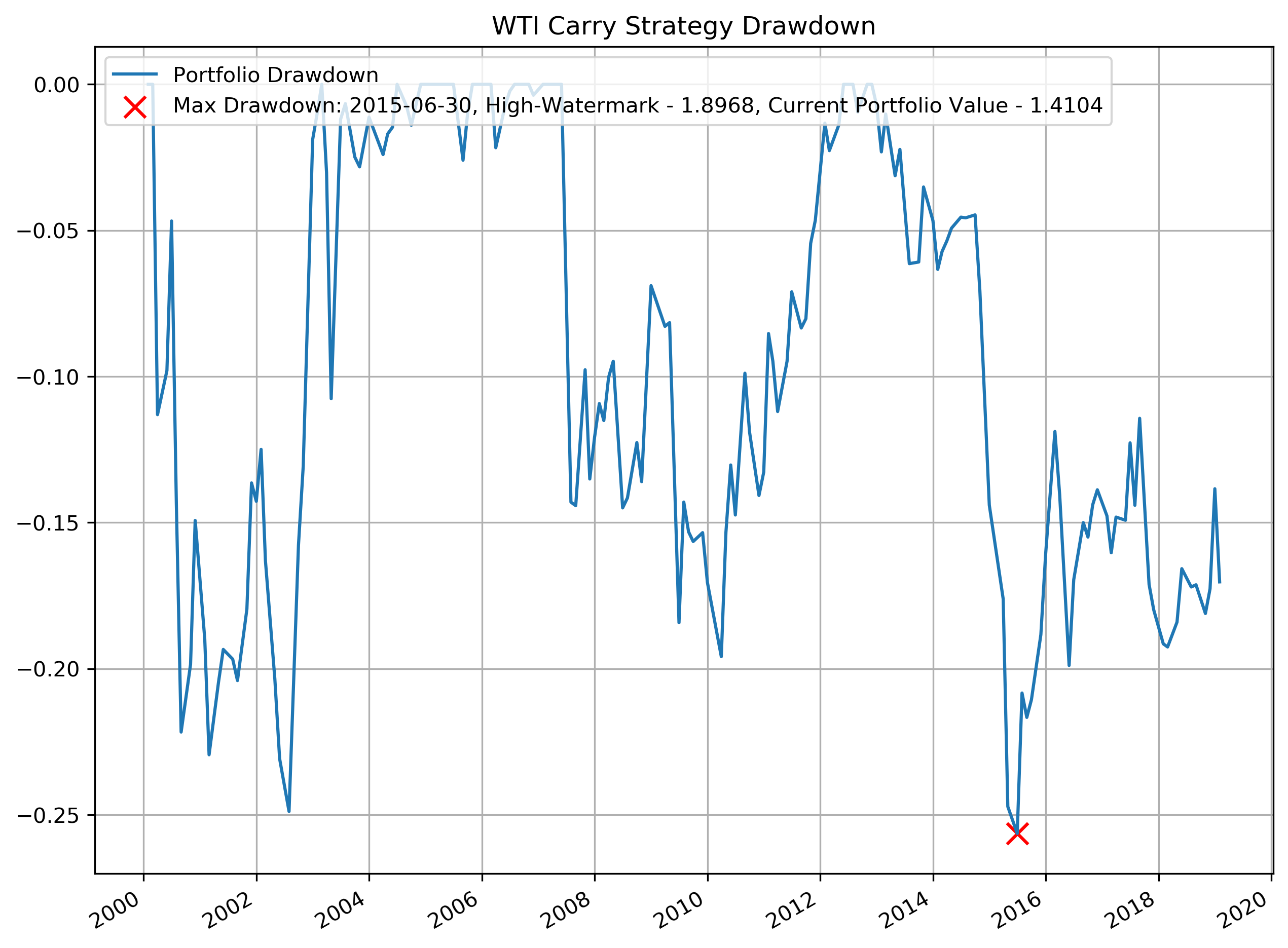
time: 745 ms