
HW 8
ISE 530 Optimization for Analytics Homework VIII: Nonlinearly constrained optimization. Due 11:59 PM Wednesday November 11, 2020.
This is derived from Exercise 11.19 in Cottle-Thapa. Define the functions \(s(t)\) and \(c(t)\) of the real variable \(t\):
Consider the nonlinear program:
Write down the KKT conditions for the problem and show that they reduce to
From a solution of the latter simplified conditions, construct a solution of the given problem?
This is derived from Exercise 11.20 in Cottle-Thapa. Write down the Karush-Kuhn-Tucker conditions of the nonlinear program:
Find a solution along with Lagrange multipliers satisfying these conditions.
Do parts (a), (b), and (c) in Exercise 11.21 in Cottle-Thapa.
Consider the nonlinear program:
Write down the Karush-Kuhn-Tucker (KKT) conditions of this problem.
Show that the linear independence constraint qualification holds at the point \((2, 1)\). Does this point satisfy the KKT conditions?
Consider a simple set in the plane consisting of points \((a, b) \geq 0\) satisfying \(ab = 0\). Show that the linear independence constraint qualification cannot hold at any feasible point in the set.
Apply the Karush-Kuhn-Tucker conditions to locate the unique of the following convex program:
Verify your solution geometrically by showing that the problem is equivalent to a closest-point problem, i.e., finding a point in the feasible region that is closest to a given point outside of the region.
Consider the following nonlinear program:
Is the objective function convex? Argue that the constraints satisfy the Slater constraint qualification. Further argue that at an optimal solution of the problem, we must have \(e^{x_1} - e^{x_2} = 20\). Use the latter fact to show that the problem is equivalent to a problem in the \(x_1\)-variable only. Solve the problem. Verify that the solution you obtain satisfies the Karush-Kuhn-Tucker conditions of the original problem in the \((x_1, x_2)\)-variables.
%load_ext autotime
%load_ext nb_black
%matplotlib inline

import matplotlib.pyplot as plt
from mpl_toolkits.mplot3d import Axes3D

plt.rcParams["figure.dpi"] = 300
plt.rcParams["figure.figsize"] = (16, 12)

import operator
import pandas as pd
import numpy as np
import cvxpy as cp
import scipy as sp
from sympy import Matrix
from scipy import optimize
This is derived from Exercise 11.19 in Cottle-Thapa. Define the functions \(s(t)\) and \(c(t)\) of the real variable \(t\):
Consider the nonlinear program:
Write down the KKT conditions for the problem and show that they reduce to
From a solution of the latter simplified conditions, construct a solution of the given problem?
KKT Conditions @ optimal \((x^*_1, x^*_2, \mu^*_1, \mu^*_2, \mu^*_3)\):
Primal Feasibility
Dual Feasibility
Complementary Slackness
Stationarity
At Optimal solution \(x^*_1 = 0, x^*_2 = 0\), our KKT conditions reduce to :
where \(u_1 = \mu^*_1, u_2 = \mu^*_2\) \(\blacksquare\)
This is derived from Exercise 11.20 in Cottle-Thapa. Write down the Karush-Kuhn-Tucker conditions of the nonlinear program:
Find a solution along with Lagrange multipliers satisfying these conditions.
KKT Conditions @ optimal \((x^*_1, x^*_2, x^*_3, \mu^*_1, \mu^*_2, \mu^*_3, \mu^*_4)\):
Primal Feasibility
Dual Feasibility
Complementary Slackness
Stationarity
Substituting Stationarity conditions into complementary slackness:
Case I: \(\mu^*_1 = 0\)
A Solution: \(x^*_1 = 1, x^*_2 = 1, x^*_3 = 1, \mu^*_1 = 0, \mu^*_2 = 40, \mu^*_3 = 57, \mu^*_4 = 20\).
Do parts (a), (b), and (c) in Exercise 11.21 in Cottle-Thapa.
Consider the optimization problem
(a) Find an optimal solution for this problem. Is it unique?
Convert to minimization problem
KKT Conditions @ optimal \((x^*_1, x^*_2, \mu^*_1, \mu^*_2, \mu^*_3)\):
Primal Feasibility
Dual Feasibility
Complementary Slackness
Stationarity
Substituting \(\mu^*_2 = 1 - 3\mu^*_1(x^*_1 - 1)^2\) and \(\mu^*_3 = \mu^*_1\) into the complementary slackness conditions:
Case I: \(x^*_1 = 1\)
Hence, this case is not possible and \(x^*_1 \not= 1\)
Case II: \(\mu^*_1 = 0\)
Optimal solution: \(x^*_1=0, x^*_2=0, \mu^*_1=0, \mu^*_2=1, \mu^*_3=0\), unique.
(b) What is the feasible region of this problem?
\(\Big\{x=\begin{bmatrix}x_1 \\x_2 \end{bmatrix}: \begin{bmatrix}x_1 \\x_2\end{bmatrix} \leq 0 \Big\}\)
(c) Is the Slater condition satisfied in this case?
Concavity of Constraints for Maximization problem:
Slater’s condition holds as when \(x\) is any vector \(< 0\).
Consider the nonlinear program:
Write down the Karush-Kuhn-Tucker (KKT) conditions of this problem.
KKT Conditions @ optimal \((x^*_1, x^*_2, \mu^*_1, \mu^*_2, \mu^*_3)\):
Primal Feasibility
Dual Feasibility
Complementary Slackness
Stationarity
Substituting \(\mu^*_2 = -1 -x^*_2 + x^*_1 + \mu^*_1 + 2\lambda^*_1 x^*_1\) and \(\mu^*_3 = -1 -x^*_1 + 2x^*_2 + 2\mu^*_1x^*_2 - \lambda^*_1\) into the complementary slackness conditions:
Show that the linear independence constraint qualification holds at the point \((2, 1)\). Does this point satisfy the KKT conditions?
Gradients of Constraints:
At \(x_1 = 2\) and \(x_2 = 1\), the following are the gradients of the active constraints:
We see that the active constraints are linearly indepdendent, hence, Linear Independence Constraint Qualifications (LICQ) holds. \(\blacksquare\)
Plugging in \(x_1 = 2\) and \(x_2 = 1\) into the KKT Stationarity conditions:
Substituting into the Complementary slackness conditions:
This indicates that the point is not dual feasible, and hence does not satisfy the KKT conditions and is hence not optimal.
Consider a simple set in the plane consisting of points \((a, b) \geq 0\) satisfying \(ab = 0\). Show that the linear independence constraint qualification cannot hold at any feasible point in the set.
If \((a, b) \geq 0\) and \(ab = 0\), it must mean that either \(a=0\) or \(b=0\) (cannot be both as it will be infeasible).
Gradients of Constraints:
For \((a, b)\) to be feasible, we need:
If only \(a = 0 \rightarrow b = -3\), violates our assumption that \((a, b) \geq 0\).
If only \(b = 0 \rightarrow a = \sqrt{3}\). However, this will mean the gradient of the active constraints will be:
which are linearly independent.
Unless \(a = \sqrt{3}, b=0\), LICQ cannot hold, given that \((a, b) \geq 0\) satisfying \(ab = 0\). \(\blacksquare\)
Apply the Karush-Kuhn-Tucker conditions to locate the unique of the following convex program:
KKT Conditions @ optimal \((x^*_1, x^*_2, \mu^*_1, \mu^*_2)\):
Primal Feasibility
Dual Feasibility
Complementary Slackness
Stationarity
Substituting \(\mu^*_2 = -2x^*_2 + 4 + \mu^*_1\) into \(2x^*_1 - 4 + 2\mu^*_1 x^*_1 + \mu^*_2 = 0\):
Substituting \(\mu^*_2 = -2x^*_2 + 4 + \mu^*_1\) into the second complementary slackness condition \(\mu^*_2 (x^*_1 + x^*_2 - 2) = 0\):
Case I: \(\mu^*_2 = 0 \rightarrow -2x^*_2 + 4 + \mu^*_1 = 0\), \(\therefore \mu^*_1 = 2x^*_2 - 4 \,\,--\,\,(2)\)
Substituting into first complementary slackness condition:
(1) = (2):
solution = sp.optimize.root(lambda x: 2 * (x[0] ** 3) - 3 * x[0] - 2, x0=[1.4])
solution
    fjac: array([[-1.]])
     fun: -1.0658141036401503e-14
 message: 'The solution converged.'
    nfev: 7
     qtf: array([-6.60441746e-09])
       r: array([-10.06588727])
  status: 1
 success: True
       x: array([1.47568652])
time: 2.75 ms
x_2_star = solution.x[0] ** 2
μ_1_star = 2 * x_2_star - 4
μ_2_star = 0
print(
    f"Optimal Solution: x^*_1={np.round(solution.x[0], 3)}, x^*_2={np.round(x_2_star, 3)}, μ^*_1={np.round(μ_1_star, 3)}, μ^*_2={np.round(μ_2_star, 3)}"
)
Optimal Solution: x^*_1=1.476, x^*_2=2.178, μ^*_1=0.355, μ^*_2=0
time: 1.36 ms
However, since \(x_1 + x_2 \leq 2\) is violated, this solution is rejected.
Case II: \(x^*_1 = -x^*_2 + 2 \,\,--\,\,(3)\)
Substituting \((3)\) into \((1)\): \(\mu^*_1 = \frac{-2(-x^*_2 + 2) + 2x^*_2}{2(-x^*_2 + 2) + 1}\) and into first complementary slackness condition:
Optimal Solution: \(x^*_1 = 1, x^*_2 = 1, \mu^*_1=0, \mu^*_2 = 2 \because \mu^*_2 = -2x^*_2 + 4 + \mu^*_1\)
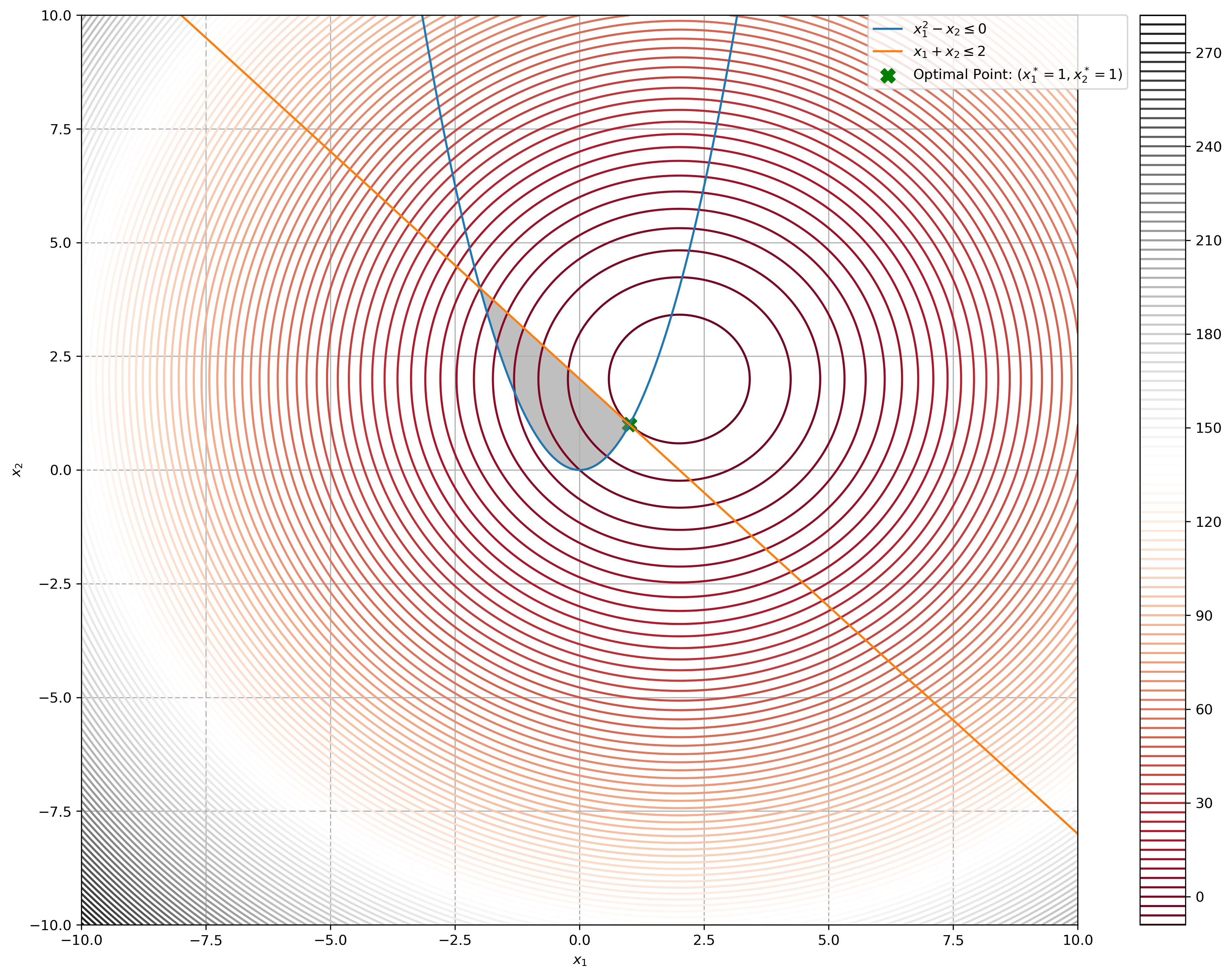
Verify your solution geometrically by showing that the problem is equivalent to a closest-point problem, i.e., finding a point in the feasible region that is closest to a given point outside of the region.
f = lambda x: x[0] ** 2 + x[1] ** 2 - 4 * x[0] - 4 * x[1]
x_1 = np.linspace(-10, 10, 1000)
x_2_1 = lambda x_1: x_1 ** 2  # 𝑥^2_1 − 𝑥_2 ≤ 0
x_2_2 = lambda x_1: 2 - x_1  # 𝑥_1 + 𝑥_2 ≤ 2

# Constraints
plt.plot(x_1, x_2_1(x_1), label=r"$x^2_1 - x_2 \leq 0$")
plt.plot(x_1, x_2_2(x_1), label=r"$x_1 + x_2 \leq 2$")

# Objective function
X_1, X_2 = np.meshgrid(x_1, x_1)
Z = f([X_1, X_2])
plt.contour(X_1, X_2, Z, 100, cmap="RdGy")
plt.colorbar()

# Optimal point
plt.scatter(
    1, 1, s=100, c="green", marker="X", label=r"Optimal Point: ($x^*_1 = 1, x^*_2 = 1$)"
)

plt.xlim((-10, 10))
plt.ylim((-10, 10))
plt.xlabel(r"$x_1$")
plt.ylabel(r"$x_2$")

# Fill feasible region
x_2_lb = np.minimum(x_2_1(x_1), x_2_2(x_1))
plt.fill_between(
    x_1, x_2_lb, x_2_2(x_1), where=x_2_2(x_1) > x_2_lb, color="grey", alpha=0.5
)
plt.grid(True)
plt.legend(bbox_to_anchor=(1.05, 1), loc="best", borderaxespad=0.0)
plt.show()
time: 2.94 s
We see that the problem is essentially finding the smallest radius of the concentric rings thatmeet both constraints at a point.
Consider the following nonlinear program:
Is the objective function convex? Argue that the constraints satisfy the Slater constraint qualification. Further argue that at an optimal solution of the problem, we must have \(e^{x_1} - e^{x_2} = 20\). Use the latter fact to show that the problem is equivalent to a problem in the \(x_1\)-variable only. Solve the problem. Verify that the solution you obtain satisfies the Karush-Kuhn-Tucker conditions of the original problem in the \((x_1, x_2)\)-variables.
Hessian of \({x_1}^2 - x_2\) is positive semi-definite, hence convex:
Exponential of convex function is strictly convex, meaning our objective function is strictly convex.
\(e^{x_1} - e^{x_2} - 20 \leq 0\) is stricly convex since exponential of affine / convex functions are strictly convex, summation is a convex operation, meaning that the constraint is convex, the other constraint \(-x_1 \leq 0\) is simply affine.
Purely by observation, we know beforehand that the infimum of \(e^{-x}\) is \(0\). We can clearly see that since \(x_2\) is free, by setting \(x_1 = 0\), and \(x_2 = \infty\), we achieve the infimum of our objective function while satisfying the constraints.
By using the equality constraint \(e^{x_1} - e^{x_2} = 20 \rightarrow x_2 = \ln{(e^{x_1} - 20)}\):
solution = sp.optimize.root(
    lambda x: -np.exp(x[0] ** 2) * np.log(np.exp(x[0]) - 20), x0=[5]
)
solution
    fjac: array([[-1.]])
     fun: -2.562096193561078e-09
 message: 'The solution converged.'
    nfev: 31
     qtf: array([0.00020205])
       r: array([222715.83895117])
  status: 1
 success: True
       x: array([3.04452244])
time: 4.22 ms
x_1_star = solution.x[0]
x_2_star = np.log(np.exp(x_1_star) - 20)
x_1_star, x_2_star
(3.0445224377234346, 2.415845301584049e-13)
time: 2.26 ms
KKT Conditions @ optimal \((x^*_1, x^*_2, \mu^*_1, \mu^*_2)\):
Primal Feasibility:
Dual Feasibility:
Complementary Slackness:
Stationarity:
μ_1_star = -np.exp(x_1_star ** 2 - x_2_star) / np.exp(x_2_star)
μ_2_star = 2 * x_1_star * np.exp(x_1_star ** 2 - x_2_star) + μ_1_star * np.exp(x_1_star)
μ_1_star, μ_2_star
(-10605.381859011817, -158136.37297846202)
time: 2.54 ms