Project 1: Momentum Strategies¶

By: Chengyi (Jeff) Chen

Description of The Project:¶

We want to test the momentum effect on different assets. We have daily price time series information for assets in the following asset classes:

Equity Index
Credit (Corporate Bonds)
Govt Bond (Sovereign Bonds)
Currencies
Commodities
Equity Factors

You choose one of the above 6 asset classes, and we’ll build momentum portfolios for each one of the assets in the chosen asset class.

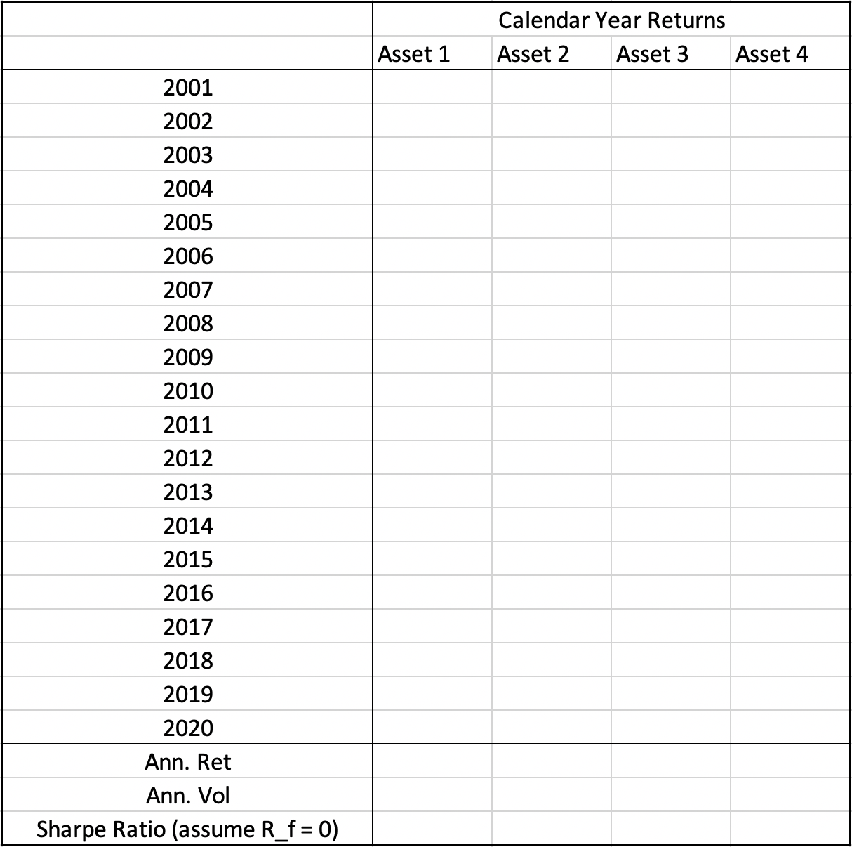
For every asset, based on its price time series, a momentum portfolio could be built in the following way: Step 1: starting from 12/31/2001, at each month-end time point, calculate the asset’s return in the past 12 months, if the return is positive (negative), the portfolio longs (shorts) 100% of the asset and holds the long (short) position for the next month. Step 2: calculate the monthly returns for the above-built portfolio till 2020/8/31. Step 3: prepare the deliverable table as follows:

Bonus problem At step 1, at each month-end date, calculate all asset returns in the past 12 months,
and allocate 50% weight to the top two performing assets respectively; and -50% to the bottom two performing assets respectively in your portfolio. And then do step 2 and step 3.

%load_ext nb_black
%load_ext autotime

import pandas as pd
import numpy as np
from typing import Dict
from datetime import datetime, timedelta
from abc import ABC, abstractmethod


def get_asset_class_data(raw_data: pd.DataFrame) -> pd.DataFrame:
    """Splits the Raw dataframe into the separate asset 
    class dataframes and return them in a MultiIndex Dataframe
    """
    asset_class_df_list = np.split(
        raw_data, np.argwhere(raw_data.isnull().all(axis=0).values).flatten(), axis=1
    )
    asset_class_dfs = {}
    for df in asset_class_df_list:
        df = df.dropna(how="all", axis=1)
        asset_class_name = df.iloc[0, 0]
        columns = df.iloc[0, :].str.cat(df.iloc[1, :], sep=" - ")
        columns.iloc[0] = "Date"
        df.columns = columns
        df = df.drop([0, 1], axis=0)
        df = df.set_index("Date")
        asset_class_dfs[
            asset_class_name
        ] = df.sort_index()  # Earliest stock price on top
    return pd.concat(asset_class_dfs, names=["asset_class", "security"], axis=1)


class TradingStrategy(ABC):
    def __init__(
        self, name: str, asset_class_history: pd.DataFrame, asset_class="Equity Idx"
    ):
        self.name = name
        self.asset_class = asset_class
        self.asset_class_history = asset_class_history

    @abstractmethod
    def execute_backtest(self):
        """"""
        pass

    @abstractmethod
    def _results(self):
        """"""
        pass

    @staticmethod
    def annualized_volatility(returns):
        returns = returns.dropna(axis=0)
        return np.std(returns) * np.sqrt(len(returns)) if len(returns) > 0 else None

    @staticmethod
    def annualized_return(returns):
        returns = returns.dropna(axis=0)
        return (
            (
                np.prod(np.ones(len(returns)) + np.array(returns)) ** (1 / len(returns))
                - 1
            )
            if len(returns) > 0
            else None
        )

    @staticmethod
    def calendar_year_return(returns):
        returns = returns.dropna(axis=0)
        return (
            ((TradingStrategy.annualized_return(returns) + 1) ** 12) - 1
            if len(returns) > 0
            else None
        )

    @staticmethod
    def sharpe_ratio(returns, R_f=0):
        returns = returns.dropna(axis=0)
        R_p = TradingStrategy.annualized_return(returns)
        σ_p = TradingStrategy.annualized_volatility(returns)
        return (R_p - R_f) / σ_p if len(returns) > 0 else None

data = get_asset_class_data(
    pd.read_excel(
        "./data/Project1_TimeSeries_Momentum_Due20200913.xlsx",
        sheet_name=2,
        header=None,
    )
)

time: 3.34 s

Time Series Momentum Strategy¶

class TimeSeriesMomentumStrategy(TradingStrategy):
    """Longs (Shorts) 100% for 1 month if asset's own past 12 month returns > 0 (< 0) 
    Assumes that all transactions happen on the end of month
    """

    def __init__(self, momentum_signal_period: int = 12, **kwargs):
        super().__init__(name="Time Series Momentum Strategy", **kwargs)
        self.momentum_signal_period = momentum_signal_period
        self.target_asset_history = self.asset_class_history[
            self.asset_class_history.columns[
                self.asset_class_history.columns.get_level_values("asset_class")
                == asset_class
            ]
        ]

    def filter_month_end(self, df):
        """Filter out only data of end of month"""
        dates = df.index
        only_month_end_df = df[pd.Series(dates, index=dates).dt.is_month_end]
        return only_month_end_df

    def check_data(self):
        """"""
        # Check if there's enough data from the past data for a momentum strategy
        try:
            self.start_date_idx = np.argwhere(
                self.only_month_end_df.index
                == datetime.strptime(self.start_date, self.date_format)
            ).flatten()[0]

            self.end_date_idx = np.argwhere(
                self.only_month_end_df.index
                == datetime.strptime(self.end_date, self.date_format)
            ).flatten()[0]
        except:
            raise ValueError(f"{start_date} not available in asset history data.")
        assert self.start_date_idx - 1 >= self.momentum_signal_period, print(
            f"There is not enough data (Number of months < {self.momentum_signal_period}) before {self.start_date} to generate a momentum signal."
        )

    def execute_backtest(
        self,
        start_date: str = "2001-12-31",
        end_date: str = "2020-08-31",
        date_format: str = "%Y-%m-%d",
    ):
        """Contains the actual trading logic """
        self.start_date = start_date
        self.end_date = end_date
        self.date_format = date_format
        self.only_month_end_df = self.filter_month_end(df=self.target_asset_history)
        self.check_data()
        self.past_12_month_returns = self.only_month_end_df.pct_change(
            self.momentum_signal_period
        ).iloc[
            self.start_date_idx : self.end_date_idx + 1
        ]  # Cumulative returns from past 12 months
        self.monthly_long_position_returns = (
            self.only_month_end_df.iloc[self.start_date_idx - 1 :]
            .pct_change(1)
            .iloc[1 : self.end_date_idx + 1]
        )  # End of Month Monthly Long position returns
        self.monthly_returns = (
            self.past_12_month_returns.apply(np.sign).shift(1).iloc[1:]
            * self.monthly_long_position_returns.iloc[1:]
        )
        self._results()

    def _results(self):
        """"""
        self.annual_results = self.monthly_returns.groupby(
            [self.monthly_returns.index.year]
        ).agg([self.calendar_year_return])
        self.asset_class_annualized_returns = self.annual_results.apply(
            self.annualized_return, axis=0
        ).droplevel(-1)
        self.asset_class_annualized_returns.name = "Annualized Returns"
        self.asset_class_annualized_volatility = (
            self.monthly_returns.groupby([self.monthly_returns.index.year])
            .agg([self.annualized_volatility])
            .apply(self.annualized_volatility, axis=0)
        ).droplevel(-1)
        self.asset_class_annualized_volatility.name = "Annualized Volatility"
        self.asset_class_sharpe_ratio = self.annual_results.apply(
            self.sharpe_ratio, axis=0
        ).droplevel(-1)
        self.asset_class_sharpe_ratio.name = "Sharpe Ratio (assuming $R_f$ = 0)"
        display(self.annual_results)
        display(
            pd.concat(
                [
                    self.asset_class_annualized_returns,
                    self.asset_class_annualized_volatility,
                    self.asset_class_sharpe_ratio,
                ],
                axis=1,
            ).transpose()
        )

time: 58.3 ms

for asset_class in data.columns.get_level_values("asset_class").unique():
    print("=" * 100)
    tsms = TimeSeriesMomentumStrategy(asset_class=asset_class, asset_class_history=data)
    tsms.execute_backtest()

====================================================================================================

	Equity Idx
	S&P 500 - SPX	Russell 2K - RTY	NASDAQ 100 - NDX	Hang Seng - HSI	Shanghai SE - SHCOMP	KOSPI - KOSPI	ASX 200 - AS51	NIKKEI - NKY	FTSE 100 - UKX	DAX - DAX	FTSE MIB - FTSEMIB	CAC - CAC	MSCI India - M1IN	MSCI Russia - M1RU	MSCI Brazil - M1BR
	calendar_year_return	calendar_year_return	calendar_year_return	calendar_year_return	calendar_year_return	calendar_year_return	calendar_year_return	calendar_year_return	calendar_year_return	calendar_year_return	calendar_year_return	calendar_year_return	calendar_year_return	calendar_year_return	calendar_year_return
Date
2002	0.088434	0.279880	0.387414	0.142797	0.135255	-0.071996	0.051451	0.169137	0.232031	0.535081	0.264682	0.353556	0.222429	0.154326	NaN
2003	0.019208	-0.086041	-0.014318	0.113109	-0.199595	-0.015477	0.009032	-0.166724	-0.008626	0.003490	0.020381	-0.058143	0.919416	0.140371	NaN
2004	0.108757	0.182753	0.106847	0.171412	-0.074865	0.137561	0.295137	0.086359	0.112444	0.073369	0.188540	0.101350	0.191084	0.054620	NaN
2005	0.049069	0.045117	-0.123204	0.084047	0.018237	0.567997	0.240955	0.278645	0.208053	0.270714	0.201198	0.269533	0.375694	0.700018	NaN
2006	0.157767	0.183298	-0.024914	0.389660	0.988308	0.060301	0.254948	0.080900	0.144439	0.219786	0.209513	0.209697	0.510044	0.555970	NaN
2007	0.055713	-0.014266	0.191648	0.433789	0.979663	0.237113	0.174193	-0.058043	0.073884	0.222892	-0.031965	0.041919	0.731106	0.245037	NaN
2008	0.330330	0.385477	0.202456	0.055844	0.227160	0.213187	0.136177	0.516562	0.108632	0.048457	0.730014	0.198327	-0.159019	0.501275	NaN
2009	-0.119551	-0.097311	-0.273061	-0.360089	-0.359757	-0.290330	-0.251316	-0.120017	-0.145776	-0.091792	-0.184650	-0.107100	-0.545699	-0.578876	NaN
2010	0.150587	0.268146	0.200588	0.085812	-0.441488	0.235763	0.029409	-0.148346	0.126689	0.160599	-0.327295	-0.115950	0.209516	0.190655	NaN
2011	0.021055	-0.293698	0.036123	-0.271779	-0.011050	-0.228118	-0.140106	-0.104074	-0.169795	-0.193300	-0.152196	-0.111474	-0.061607	-0.317564	-0.534078
2012	0.068127	0.051368	0.183478	-0.103584	-0.094842	-0.012624	0.026742	-0.029484	0.066475	-0.097605	0.004187	-0.053662	-0.332252	-0.249583	-0.079200
2013	0.323742	0.388219	0.369096	0.065616	0.069251	0.019623	0.219773	0.593699	0.186501	0.254817	-0.006969	0.222258	-0.396076	-0.092174	-0.058150
2014	0.136783	0.048962	0.193963	-0.021945	0.624548	-0.016952	0.071487	0.089566	0.007179	0.026527	0.029781	0.025418	0.048017	0.137143	-0.070510
2015	-0.143971	-0.044132	0.097507	-0.086906	0.111542	0.002824	0.100783	0.109935	-0.024950	0.095605	0.157532	0.119448	-0.055465	-0.141711	0.516565
2016	-0.020077	-0.020325	-0.143435	-0.130668	-0.303595	-0.057955	-0.028356	-0.324395	0.043638	-0.225592	-0.217988	-0.150836	-0.182770	0.186032	-0.466803
2017	0.218228	0.146277	0.329921	0.412730	0.049283	0.239290	0.134067	0.213360	0.119541	0.125126	0.244154	0.125445	0.271831	0.052043	0.241117
2018	-0.043918	-0.110274	0.000368	-0.170337	-0.044080	0.060109	-0.014635	-0.103034	0.009453	-0.031980	0.036292	0.054855	-0.245235	-0.003945	-0.524253
2019	0.050027	-0.222140	0.394574	-0.177570	-0.254777	0.020049	0.156804	-0.174382	-0.038051	-0.139648	-0.089326	-0.078987	-0.074335	0.128606	-0.065489
2020	-0.219109	-0.324053	0.648726	-0.103680	0.079134	0.181846	-0.497120	-0.374425	-0.107319	-0.505415	-0.514804	-0.486342	-0.668994	-0.635793	0.124278

	Equity Idx
	S&P 500 - SPX	Russell 2K - RTY	NASDAQ 100 - NDX	Hang Seng - HSI	Shanghai SE - SHCOMP	KOSPI - KOSPI	ASX 200 - AS51	NIKKEI - NKY	FTSE 100 - UKX	DAX - DAX	FTSE MIB - FTSEMIB	CAC - CAC	MSCI India - M1IN	MSCI Russia - M1RU	MSCI Brazil - M1BR
Annualized Returns	0.055576	0.019841	0.124717	0.005114	0.019207	0.051567	0.030362	-0.000177	0.043581	0.012956	-0.004439	0.009452	-0.044851	-0.011820	-0.153728
Annualized Volatility	0.250217	0.258396	0.299556	0.279455	0.396346	0.309805	0.180394	0.215803	0.201919	0.342666	0.298922	0.263166	0.399527	0.422950	0.262285
Sharpe Ratio (assuming $R_f$ = 0)	0.091799	0.022376	0.132030	0.005419	0.011392	0.063658	0.037631	-0.000164	0.089658	0.013405	-0.003924	0.011559	-0.025470	-0.008077	-0.149786

====================================================================================================

	Credit
	US IG - LUACTRUU	US HY - H0A0	EU IG - SPEZICUT	EU HY - HE00	EM Corp - EMCB
	calendar_year_return	calendar_year_return	calendar_year_return	calendar_year_return	calendar_year_return
Date
2002	0.101171	-0.114729	NaN	0.033558	0.107632
2003	0.082424	0.206790	NaN	0.130784	0.171954
2004	0.044620	0.108698	NaN	0.145615	0.100654
2005	0.016762	0.027381	NaN	0.059634	0.043976
2006	0.013826	0.117671	NaN	0.111028	0.076199
2007	0.045608	0.021929	NaN	-0.022205	0.049376
2008	-0.129893	0.258021	NaN	0.436900	0.013024
2009	0.064239	-0.188552	NaN	-0.256437	-0.155023
2010	0.089958	0.151904	NaN	0.142566	0.114395
2011	0.081460	0.043827	NaN	-0.110336	-0.056776
2012	0.098174	0.155834	NaN	0.115463	0.157965
2013	-0.036943	0.074187	NaN	0.100641	-0.005148
2014	0.036368	0.025033	NaN	0.054770	-0.016850
2015	-0.021545	0.060394	NaN	0.007552	0.051350
2016	-0.019228	-0.020808	-0.066869	-0.012205	0.092452
2017	0.064178	0.074832	0.025810	0.067444	0.081342
2018	-0.040784	-0.022649	0.000440	0.010756	-0.030833
2019	0.092737	0.043631	-0.091023	0.025470	0.069415
2020	0.105935	-0.318564	-0.265735	-0.364253	-0.034163

	Credit
	US IG - LUACTRUU	US HY - H0A0	EU IG - SPEZICUT	EU HY - HE00	EM Corp - EMCB
Annualized Returns	0.034379	0.027816	-0.085631	0.022193	0.040705
Annualized Volatility	0.110831	0.211764	0.021668	0.250086	0.209394
Sharpe Ratio (assuming $R_f$ = 0)	0.128956	0.048584	-0.373882	0.031851	0.119703

====================================================================================================

	Govt Bond
	US Treasury - LUATTRUU	UK Gilt - JFBG3GUS	German Bund - CBKIG0FT	Japan JGB - SPJGBTR	EM Govt - GBIEMCOR
	calendar_year_return	calendar_year_return	calendar_year_return	calendar_year_return	calendar_year_return
Date
2002	0.117935	0.066458	0.105547	0.051543	NaN
2003	0.022414	0.006415	0.020399	-0.041043	NaN
2004	0.007724	0.003808	0.042187	0.005642	NaN
2005	0.027919	0.028276	0.042376	0.006645	NaN
2006	-0.001478	-0.030992	-0.051699	-0.013907	NaN
2007	0.090124	-0.005503	0.020445	0.040500	NaN
2008	0.137371	0.104842	-0.027833	0.035918	NaN
2009	-0.035674	-0.032949	-0.000288	0.025105	-0.088812
2010	0.004481	0.047323	0.027167	0.024459	0.154323
2011	0.098133	0.150250	0.052122	0.027175	-0.125680
2012	0.019934	0.051032	0.067543	0.018526	-0.179821
2013	0.007119	0.053977	-0.021530	0.004020	-0.070201
2014	-0.007403	0.050203	0.077912	0.040626	-0.063224
2015	0.008425	0.005043	0.020838	0.014520	0.155773
2016	0.010376	0.038564	0.070891	0.010483	-0.165256
2017	-0.015598	0.037761	-0.047833	-0.013668	0.146637
2018	-0.065910	-0.012898	0.004869	0.014964	-0.024602
2019	0.068576	0.047258	0.048424	-0.003778	-0.063896
2020	0.134123	0.074121	0.042626	-0.024609	-0.350187

	Govt Bond
	US Treasury - LUATTRUU	UK Gilt - JFBG3GUS	German Bund - CBKIG0FT	Japan JGB - SPJGBTR	EM Govt - GBIEMCOR
Annualized Returns	0.031570	0.035009	0.025165	0.011475	-0.067697
Annualized Volatility	0.055405	0.073377	0.049919	0.043905	0.084537
Sharpe Ratio (assuming $R_f$ = 0)	0.128530	0.180850	0.139315	0.113346	-0.135072

====================================================================================================

	Currencies
	EUR/USD - EURUSD	JPY/USD - JPYUSD	GBP/USD - GBPUSD	AUD/USD - AUDUSD	CNY/USD - CNYUSD
	calendar_year_return	calendar_year_return	calendar_year_return	calendar_year_return	calendar_year_return
Date
2002	0.148162	-0.077826	0.150727	0.006712	-0.000331
2003	0.200438	0.053686	0.109193	0.339031	-0.000083
2004	0.076141	0.044709	0.074140	0.037633	-0.000166
2005	-0.102000	-0.064387	-0.046275	-0.021218	-0.018382
2006	-0.050245	-0.045898	-0.039035	-0.094061	0.033091
2007	0.105479	0.003912	0.013376	0.109829	0.069609
2008	-0.044681	0.231672	0.347671	-0.009721	0.070411
2009	-0.080276	-0.024317	-0.139300	-0.216322	-0.000819
2010	-0.223406	0.046534	-0.167473	0.139913	0.034906
2011	-0.100326	0.055019	-0.113537	-0.166821	0.047657
2012	-0.025019	0.088735	-0.037251	-0.068677	0.011026
2013	0.049704	0.204304	-0.144734	0.146359	0.029040
2014	-0.012627	0.127919	-0.008513	-0.066779	-0.028018
2015	0.100158	0.000587	0.049289	0.110821	0.042214
2016	-0.078979	-0.102517	0.177952	-0.111267	0.068763
2017	-0.004080	0.030011	-0.074729	0.028235	-0.039351
2018	-0.007993	-0.023951	0.009791	-0.007616	-0.034823
2019	0.020213	-0.047243	0.002487	-0.001233	0.009126
2020	-0.056399	-0.020593	-0.053442	0.002394	-0.026229

	Currencies
	EUR/USD - EURUSD	JPY/USD - JPYUSD	GBP/USD - GBPUSD	AUD/USD - AUDUSD	CNY/USD - CNYUSD
Annualized Returns	-0.009381	0.021707	-0.001322	0.001016	0.013498
Annualized Volatility	0.136584	0.133411	0.074319	0.168132	0.073629
Sharpe Ratio (assuming $R_f$ = 0)	-0.021918	0.056978	-0.002456	0.001898	0.089492

====================================================================================================

	Commod
	WTI Oil - CL1 COMB	Brent Oil - CO1	Gold - XAUUSD	Silver - XAG	Copper - SPGSIC	Agriculture - BCOMAGTR
	calendar_year_return	calendar_year_return	calendar_year_return	calendar_year_return	calendar_year_return	calendar_year_return
Date
2002	-0.137678	-0.142562	0.247715	-0.073021	-0.196890	0.041818
2003	-0.218048	-0.163959	0.193650	-0.131105	0.081011	-0.015321
2004	0.131023	0.136938	0.055362	0.148569	0.389583	-0.165351
2005	0.404833	0.457736	0.179154	0.370638	0.401533	-0.238630
2006	-0.016730	0.152491	0.231528	0.463982	0.408749	0.108420
2007	-0.038936	0.007421	0.309408	-0.137633	-0.053572	0.298885
2008	-0.001325	-0.056533	-0.185666	-0.181195	0.671353	-0.012467
2009	-0.473938	-0.434962	0.305817	-0.231319	-0.515501	-0.009318
2010	0.151462	0.215835	0.295739	0.831556	0.308329	0.003032
2011	-0.243198	0.133298	0.100964	-0.099410	-0.342450	-0.105827
2012	-0.105795	0.074718	-0.073634	-0.421993	-0.183567	-0.257674
2013	0.055780	0.264209	0.321928	0.517521	0.116259	0.001788
2014	0.600033	0.705686	-0.068142	0.007230	0.138502	-0.026743
2015	0.230527	0.279488	-0.021973	0.095398	0.278538	0.138459
2016	-0.229107	-0.271858	-0.217889	-0.522722	-0.275194	0.011708
2017	0.032603	-0.034583	0.006521	0.005963	0.308171	0.051301
2018	-0.065707	-0.048602	-0.106186	0.126177	-0.091015	0.098412
2019	-0.163310	-0.072973	0.139826	0.035179	-0.050574	-0.036729
2020	-0.940855	-0.506588	0.476989	0.597779	-0.154135	-0.062749

	Commod
	WTI Oil - CL1 COMB	Brent Oil - CO1	Gold - XAUUSD	Silver - XAG	Copper - SPGSIC	Agriculture - BCOMAGTR
Annualized Returns	-0.166098	-0.004430	0.098833	0.019317	0.019451	-0.017449
Annualized Volatility	0.794941	0.562311	0.221906	0.509008	0.387265	0.309227
Sharpe Ratio (assuming $R_f$ = 0)	-0.120575	-0.003592	0.120173	0.013014	0.014807	-0.031794

====================================================================================================

	EQ Factors
	Value - DJTMNSV	Size - DJTMNSS	Quality - DJTMNQU	Momentum - DJTMNMO	Low Beta - DJTMNAB
	calendar_year_return	calendar_year_return	calendar_year_return	calendar_year_return	calendar_year_return
Date
2002	NaN	NaN	NaN	NaN	NaN
2003	0.128332	-0.045934	-0.027136	-0.114272	-0.095846
2004	0.124360	0.089198	-0.016135	-0.021923	-0.020721
2005	0.015967	0.022662	0.042710	0.151704	-0.007309
2006	-0.067420	0.045008	0.006538	-0.000067	-0.155052
2007	0.064438	0.014825	0.073109	0.202739	-0.000901
2008	-0.084118	0.002846	0.159003	0.080683	0.351417
2009	0.339859	0.151237	-0.060329	-0.092819	-0.164237
2010	-0.066073	0.119517	0.051802	-0.000386	0.153621
2011	0.032565	0.015253	0.089126	0.067082	-0.299770
2012	0.083043	0.032431	0.037111	0.076830	-0.060622
2013	0.158641	0.063753	-0.003690	0.003273	0.030478
2014	0.024173	-0.068263	-0.110608	-0.003507	-0.013651
2015	-0.022226	0.051858	0.103951	0.013864	0.083934
2016	0.077949	-0.059151	-0.121989	-0.008552	-0.018173
2017	-0.087912	-0.076334	0.100932	-0.038273	0.007228
2018	0.140675	0.048635	0.044165	0.057604	0.050381
2019	-0.012805	-0.017005	0.004608	-0.199652	0.030855
2020	0.712308	0.276804	-0.165403	0.132956	0.142463

	EQ Factors
	Value - DJTMNSV	Size - DJTMNSS	Quality - DJTMNQU	Momentum - DJTMNMO	Low Beta - DJTMNAB
Annualized Returns	0.073872	0.033848	0.008022	0.012581	-0.008529
Annualized Volatility	0.146757	0.111505	0.153330	0.291844	0.232533
Sharpe Ratio (assuming $R_f$ = 0)	0.094764	0.095148	0.022765	0.031399	-0.014766

time: 1.35 s

Cross-sectional Momentum Strategy¶

class CrossSectionalMomentumStrategy(TimeSeriesMomentumStrategy):
    """Longs 50% of best performing asset in past 12 months in asset class 
    and Shorts 50% of worst performing asset in past 12 months in asset class for 1 month  
    Assumes that all transactions happen on the end of month
    """

    def __init__(self, momentum_signal_period: int = 12, **kwargs):
        TradingStrategy.__init__(
            self, name="Cross Sectional Momentum Strategy", **kwargs
        )
        self.momentum_signal_period = momentum_signal_period
        self.target_asset_history = self.asset_class_history[
            self.asset_class_history.columns[
                self.asset_class_history.columns.get_level_values("asset_class")
                == asset_class
            ]
        ]

    def execute_backtest(
        self,
        start_date: str = "2001-12-31",
        end_date: str = "2020-08-31",
        date_format: str = "%Y-%m-%d",
    ):
        """Contains the actual trading logic """
        self.start_date = start_date
        self.end_date = end_date
        self.date_format = date_format
        self.only_month_end_df = self.filter_month_end(df=self.target_asset_history)
        self.check_data()
        self.past_12_month_returns = self.only_month_end_df.pct_change(
            self.momentum_signal_period
        ).iloc[
            self.start_date_idx : self.end_date_idx + 1
        ]  # Cumulative returns from past 12 months
        self.monthly_long_position_returns = (
            self.only_month_end_df.iloc[self.start_date_idx - 1 :]
            .pct_change(1)
            .iloc[1 : self.end_date_idx + 1]
        )  # End of Month Monthly Long position returns

        long_portfolio_returns = (
            self.past_12_month_returns.apply(lambda row: (row == np.max(row)), axis=1)
            .shift(1)
            .iloc[1:]
            * self.monthly_long_position_returns.iloc[1:]
        ).sum(
            axis=1
        )  # Longs 50% of best performing asset in past 12 months in asset class

        short_portfolio_returns = -(
            self.past_12_month_returns.apply(lambda row: (row == np.min(row)), axis=1)
            .shift(1)
            .iloc[1:]
            * self.monthly_long_position_returns.iloc[1:]
        ).sum(
            axis=1
        )  # Shorts 50% of worst performing asset in past 12 months in asset class

        self.monthly_returns = (
            long_portfolio_returns * 0.5 + short_portfolio_returns * 0.5
        )  # Weight portfolios
        self._results()

    def _results(self):
        """"""
        self.annual_results = self.monthly_returns.groupby(
            [self.monthly_returns.index.year]
        ).agg([self.calendar_year_return])
        self.asset_class_annualized_returns = pd.Series(
            self.annual_results.apply(self.annualized_return, axis=0).values,
            name="Annualized Returns",
        )
        self.asset_class_annualized_volatility = pd.Series(
            (
                self.monthly_returns.groupby([self.monthly_returns.index.year])
                .agg([self.annualized_volatility])
                .apply(self.annualized_volatility, axis=0)
            ).values,
            name="Annualized Volatility",
        )
        self.asset_class_sharpe_ratio = pd.Series(
            self.annual_results.apply(self.sharpe_ratio, axis=0).values,
            name="Sharpe Ratio (assuming $R_f$ = 0)",
        )
        self.annual_results = self.annual_results.style.set_caption(self.asset_class)
        display(self.annual_results)
        summary = pd.concat(
            [
                self.asset_class_annualized_returns,
                self.asset_class_annualized_volatility,
                self.asset_class_sharpe_ratio,
            ],
            axis=1,
        ).transpose()
        summary.columns = ["Summary"]
        display(summary)

time: 63 ms

for asset_class in data.columns.get_level_values("asset_class").unique():
    print("=" * 100)
    csms = CrossSectionalMomentumStrategy(
        asset_class=asset_class, asset_class_history=data
    )
    csms.execute_backtest()

====================================================================================================

Equity Idx
	calendar_year_return
Date
2002	0.099955
2003	0.175910
2004	0.076786
2005	0.200651
2006	0.306280
2007	0.417425
2008	-0.139295
2009	-0.365068
2010	-0.063702
2011	-0.007779
2012	-0.043413
2013	0.113152
2014	-0.019550
2015	0.138860
2016	-0.247295
2017	0.008662
2018	-0.214263
2019	-0.030656
2020	0.345217

	Summary
Annualized Returns	0.019892
Annualized Volatility	0.163184
Sharpe Ratio (assuming $R_f$ = 0)	0.023065

====================================================================================================

Credit
	calendar_year_return
Date
2002	0.062447
2003	-0.020326
2004	0.034811
2005	0.003829
2006	0.036200
2007	0.013033
2008	0.114485
2009	-0.156851
2010	0.038716
2011	-0.028698
2012	-0.006391
2013	0.057092
2014	-0.000328
2015	-0.002702
2016	0.027312
2017	-0.016831
2018	-0.009025
2019	0.041674
2020	0.004932

	Summary
Annualized Returns	0.008773
Annualized Volatility	0.074868
Sharpe Ratio (assuming $R_f$ = 0)	0.038750

====================================================================================================

Govt Bond
	calendar_year_return
Date
2002	0.014456
2003	-0.020465
2004	0.000196
2005	0.008041
2006	0.013660
2007	0.053238
2008	0.012984
2009	-0.079125
2010	0.031045
2011	-0.068423
2012	-0.023359
2013	-0.007865
2014	0.039288
2015	0.070262
2016	-0.044730
2017	0.049316
2018	-0.030712
2019	-0.015553
2020	-0.049961

	Summary
Annualized Returns	-0.003329
Annualized Volatility	0.097833
Sharpe Ratio (assuming $R_f$ = 0)	-0.018946

====================================================================================================

Currencies
	calendar_year_return
Date
2002	0.024058
2003	0.094440
2004	-0.013657
2005	-0.036125
2006	-0.001895
2007	0.000725
2008	0.099092
2009	-0.106025
2010	-0.049425
2011	-0.041039
2012	-0.032922
2013	0.090975
2014	-0.011465
2015	-0.009285
2016	0.059619
2017	0.029123
2018	-0.028743
2019	-0.014778
2020	-0.036071

	Summary
Annualized Returns	-0.000491
Annualized Volatility	0.070615
Sharpe Ratio (assuming $R_f$ = 0)	-0.002142

====================================================================================================

Commod
	calendar_year_return
Date
2002	-0.044172
2003	-0.148021
2004	0.005226
2005	0.168395
2006	0.228971
2007	0.049709
2008	0.356241
2009	-0.290566
2010	0.018869
2011	0.036266
2012	-0.201700
2013	0.165785
2014	0.110457
2015	0.035128
2016	-0.308718
2017	0.019870
2018	-0.112933
2019	-0.099779
2020	-0.442822

	Summary
Annualized Returns	-0.044557
Annualized Volatility	0.381381
Sharpe Ratio (assuming $R_f$ = 0)	-0.053051

====================================================================================================

EQ Factors
	calendar_year_return
Date
2002	0.000000
2003	-0.021777
2004	-0.035077
2005	0.023022
2006	-0.033745
2007	0.061733
2008	0.018270
2009	0.016557
2010	-0.011831
2011	-0.175542
2012	0.014983
2013	0.110600
2014	-0.079264
2015	0.058069
2016	-0.072724
2017	0.009679
2018	0.037166
2019	0.026270
2020	0.427873

	Summary
Annualized Returns	0.014129
Annualized Volatility	0.228858
Sharpe Ratio (assuming $R_f$ = 0)	0.028603

time: 1.04 s

ΨΦ

Project 1: Momentum Strategies¶

Description of The Project:¶

Time Series Momentum Strategy¶

Cross-sectional Momentum Strategy¶